Marketing Mix Modeling for Digital vs Offline Media

marketing mix models

An analysis of FourTex’s marketing mix model showing that Facebook and Google drive the strongest website traffic returns, while TV and radio contribute little to this specific performance outcome.

Author

Ceren Unal

1 Introduction

FourTex is an apparel brand. Its products are targeted at the mass market with a focus on casual apparel for men and women. The brand’s advertising is prominent and extensive, and is present on multiple channels such as television, radio, paid search, and social media.

Recently, the digital marketing tools have extended FourTex’s reach among the potential customers. The marketing director, Hannah Schmidt, was so proud of her team’s achievements. She was getting ready for a meeting with the management board to explain how successful their previous marketing campaigns were, and hoping to get some additional budget in order to further improve the brand’s online store visits and sales leads performance metrics.

The meeting did not go as planned. In a difficult conversation, the chief executive officer (CEO) of the company said: “Mrs. Schmidt, you always ask for more money, but can rarely explain how much incremental value this money will generate”. Coming out of the meeting, Mrs. Schmidt felt that she was under enormous pressure to demonstrate the value of her marketing decisions.

Next day, she pulled some data from the company’s database, taking her notes. The table below provides a brief description of her data set:

Marketing_Mix_Variable	Description	Channel
Google AdWords	Cost of Google AdWords campaigns	Online
Facebook ads	Cost of sponsered ads delivered on Facebook	Online
TV ads	Cost of TV advertising	Offline
Radio ads	Cost of radio advertising	Offline
Web traffic	Total number of visits to the website	Online

Being very keen to demonstrate marketing’s value, Mrs. Schmidt asked her analytics team to assess the impact of their Google AdWords, Facebook, TV, and radio ads on website traffic performance. She did not want to include the sales performance metric in the analysis because her campaigns last year aimed to increase conversion to the website rather than the sales outcomes. Therefore, she thought that the relevant key performance indicator was website traffic.

Finally, Mrs. Schmidt prepared a checklist for the analytics team. She seeks answers to the following questions:

Which marketing mix instrument really drives the performance outcome, i.e. website traffic?
What is the return on marketing investment?
Should I keep pushing on with Google adwords and Facebook ads? Should I stop advertising on TV and radio channels?

How can Mrs. Schmidt demonstrate the impact of her marketing mix decisions to the management board?

To address Mrs. Schmidt’s questions, we will build a marketing mix model that gauges the effectiveness of her marketing mix decisions and estimates the contribution of each advertising vehicle to website traffic performance.

Before we roll out the analyses, we should make sure that all our files are organised and our R environment is set up.

2 Preparation and set-up

3 Exploratory data analysis

3.1 Packages

Code

library(tidyverse)
library(janitor)
library(scales)
theme_set(theme_light())

3.2 Data

Code

data <- read_csv("data/data_fourtex.csv")
str(data)

spc_tbl_ [57 × 6] (S3: spec_tbl_df/tbl_df/tbl/data.frame)
 $ week_beg      : chr [1:57] "06/07/2020" "13/07/2020" "20/07/2020" "27/07/2020" ...
 $ Google_Adwords: num [1:57] 94017 93635 112239 121250 130471 ...
 $ Facebook      : num [1:57] 82950 66150 94650 96450 114600 ...
 $ TV            : num [1:57] 0 0 0 0 0 0 0 0 0 0 ...
 $ Radio         : num [1:57] 0 0 0 0 0 ...
 $ traffic       : num [1:57] 6719812 6186229 6790416 7146957 7815741 ...
 - attr(*, "spec")=
  .. cols(
  ..   week_beg = col_character(),
  ..   Google_Adwords = col_double(),
  ..   Facebook = col_double(),
  ..   TV = col_double(),
  ..   Radio = col_double(),
  ..   traffic = col_double()
  .. )
 - attr(*, "problems")=<externalptr>

Code

class(data)

[1] "spec_tbl_df" "tbl_df"      "tbl"         "data.frame"

Code

data <- data |> clean_names()

The data set has 6 variables and 57 time series observations for each variable.

Next, we would like to extract each of the variables to the environment tab:

Code

# Extract the variables
google_adwords <- data$google_adwords
facebook <- data$facebook
tv <- data$tv
radio <- data$radio
traffic <- data$traffic

Code

# Make the data time series data in R
# Frequency=52
google_adwords <- ts(google_adwords, frequency = 52, start = c(2020, 28))
facebook <- ts(facebook, frequency = 52, start = c(2020, 28))
tv <- ts(tv, frequency = 52, start = c(2020, 28))
radio <- ts(radio, frequency = 52, start = c(2020, 28))
traffic <- ts(traffic, frequency = 52, start = c(2020, 28))

Important

Setting ts() arguments

Note that the dataset runs on a weekly basis. We set the frequency of the data to weeks. However, not all the years have weeks. Normally, the year has 365.25/7 = 52.18 weeks, on average. This allows for a leap year every fourth year. Therefore, some years may have 53 weeks. This is not an issue for our data, as we have 57 observations spanning over two years. None of them covers 53 weeks.

3.3 Plot the data

To get a feel for the data patterns, we need to perform a visual inspection through time series plots. First, we sum up online spending variables to find the total online spending. We do the same for offline spending variables.

Code

online_total <- google_adwords + facebook
offline_total <- tv + radio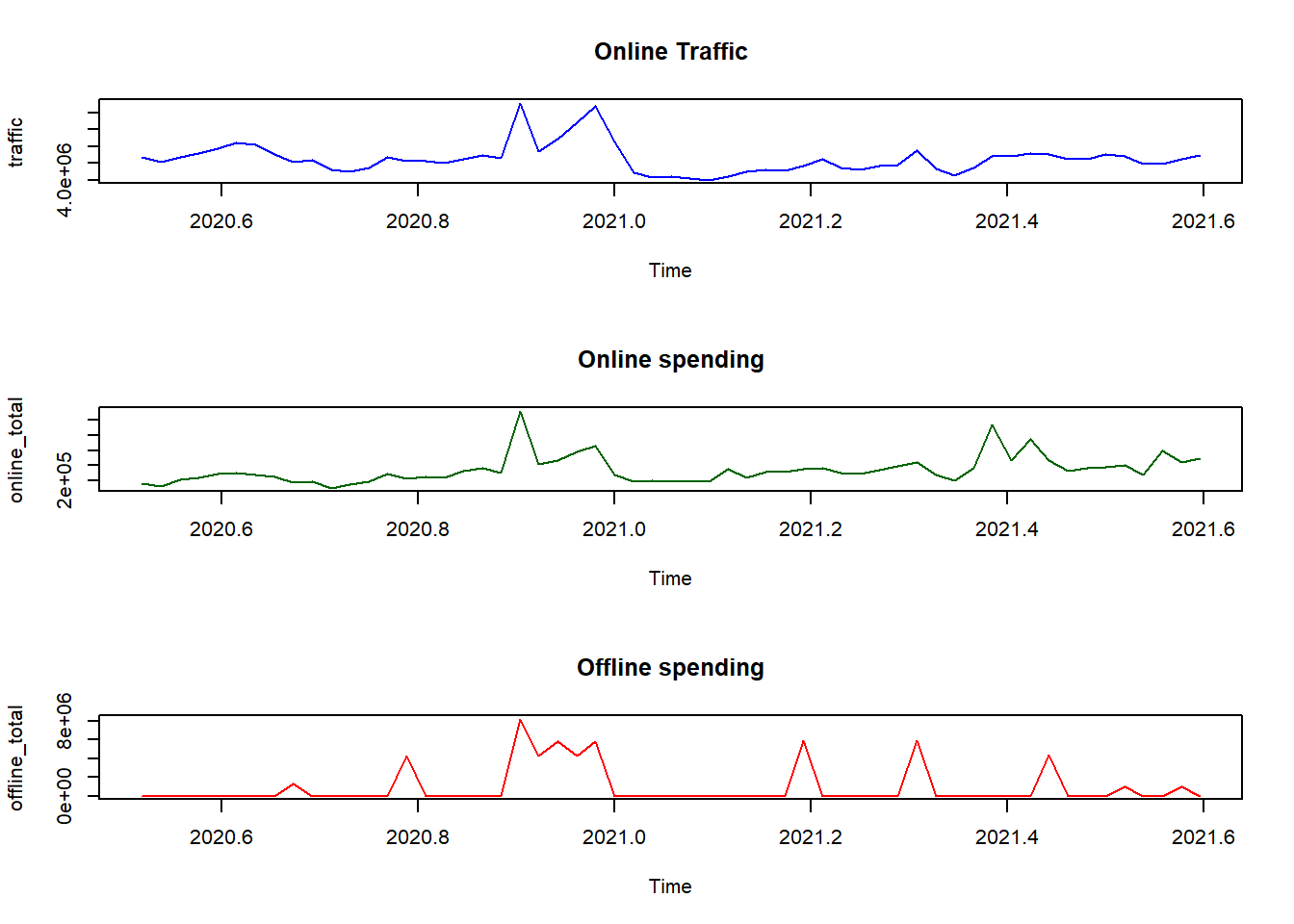

Code

par(mfrow = c(3, 1))
plot(traffic, col = "blue", main = "Online Traffic")
plot(online_total, col = "darkgreen", main = "Online spending")
plot(offline_total, col = "red", main = "Offline spending")

3.4 Current Budget allocation

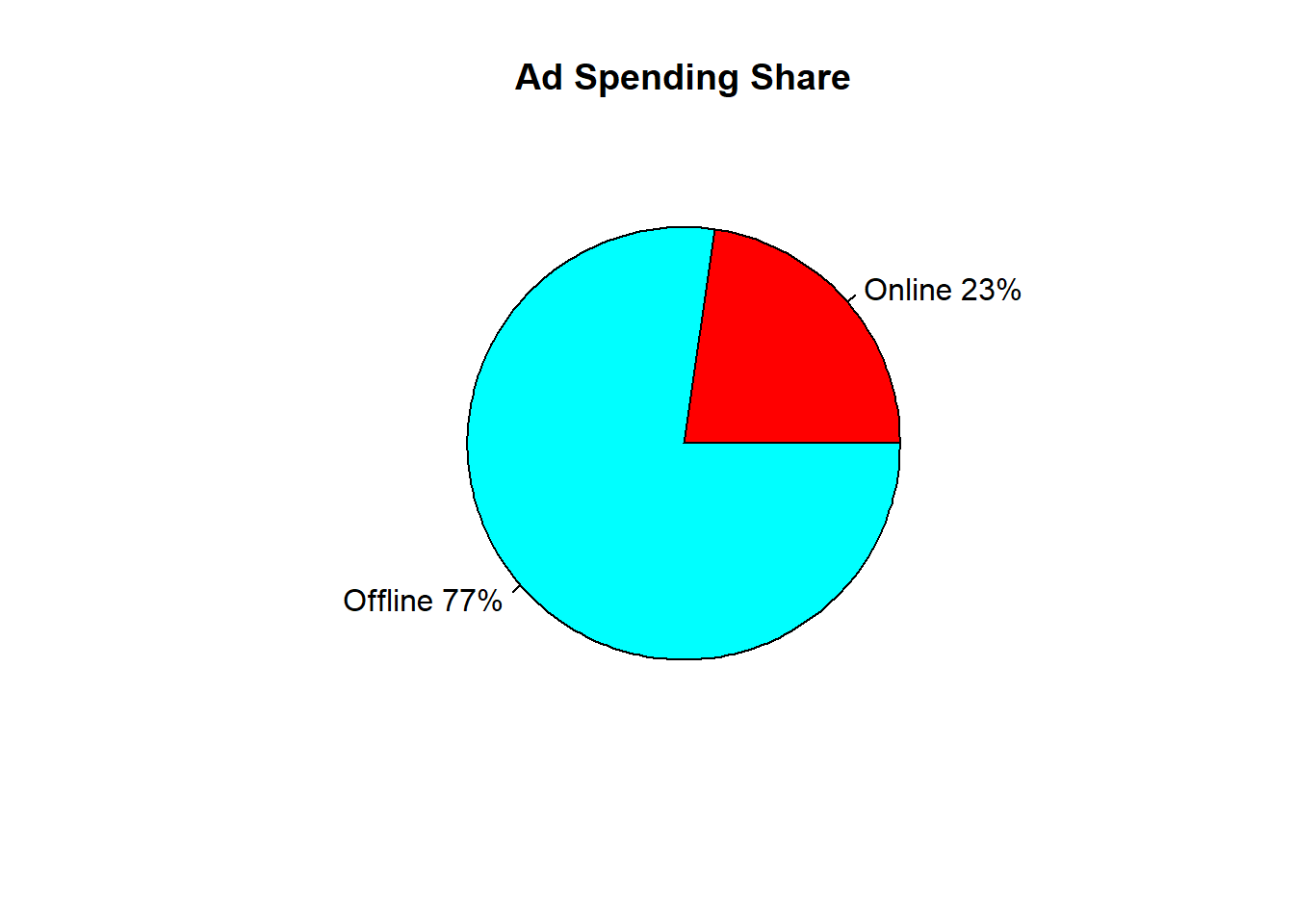
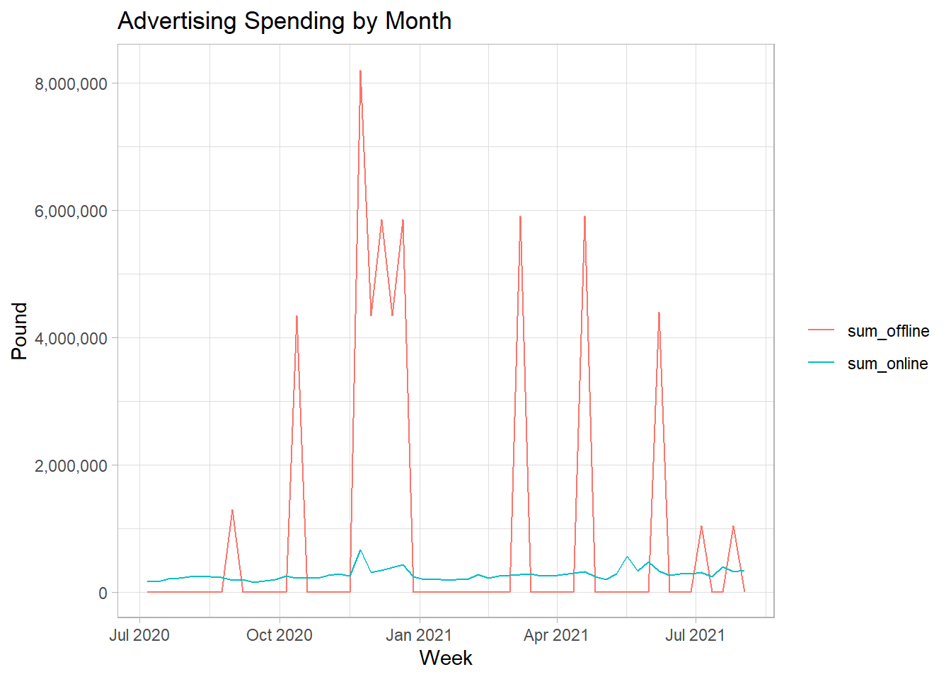
Next, we will have a look at the current budget allocation of online vs. traditional media spending.

Pie chart

Code

### Media spending share
sum_online <- sum(online_total)
sum_offline <- sum(offline_total)
total_spend <- sum_online + sum_offline

online_share <- sum_online / total_spend
offline_share <- sum_offline / total_spend

### Pie-Chart for Media Spending Share
slices <- c(online_share, offline_share)
lbls <- c("Online", "Offline")
pct <- round(slices * 100)
lbls <- paste(lbls, pct) # add percent data to labels
lbls <- paste(lbls, "%", sep = "") # add % sign to labels
par(mfrow = c(1, 1))
pie(
  slices,
  labels = lbls,
  col = rainbow(length(lbls)),
  main = "Ad Spending Share"
)

Line chart

Code

library(lubridate)
data <- data |>
  mutate(
    google_adwords = ts(google_adwords, frequency = 52, start = c(2020, 28)),
    facebook = ts(facebook, frequency = 52, start = c(2020, 28)),
    tv = ts(tv, frequency = 52, start = c(2020, 28)),
    radio = ts(radio, frequency = 52, start = c(2020, 28))
  ) |>
  mutate(sum_online = google_adwords + facebook, sum_offline = tv + radio) |>
  mutate(week_beg = dmy(week_beg))

library(scales)
data |>
  pivot_longer(
    c(sum_online, sum_offline),
    names_to = "type",
    values_to = "amount"
  ) |>
  ggplot(aes(week_beg, amount, group = type)) +
  geom_line(aes(color = type)) +
  scale_y_continuous(labels = comma_format()) +
  labs(
    title = "Advertising Spending by Month",
    x = "Week",
    y = "Pound",
    color = ""
  )

Bar chart

Code

data |>
  summarize(online = sum(sum_online), offline = sum(sum_offline)) |>
  pivot_longer(everything(), names_to = "ad_type", values_to = "amount") |>
  mutate(percent = amount / sum(amount)) |>
  ggplot(aes(ad_type, amount, fill = ad_type)) +
  geom_col(show.legend = FALSE) +
  geom_text(
    aes(label = paste0(round(percent * 100, digits = 2), "%")),
    vjust = -0.4
  ) +
  scale_y_continuous(labels = comma_format()) +
  labs(title = "Advertising Spending by Type of Ads")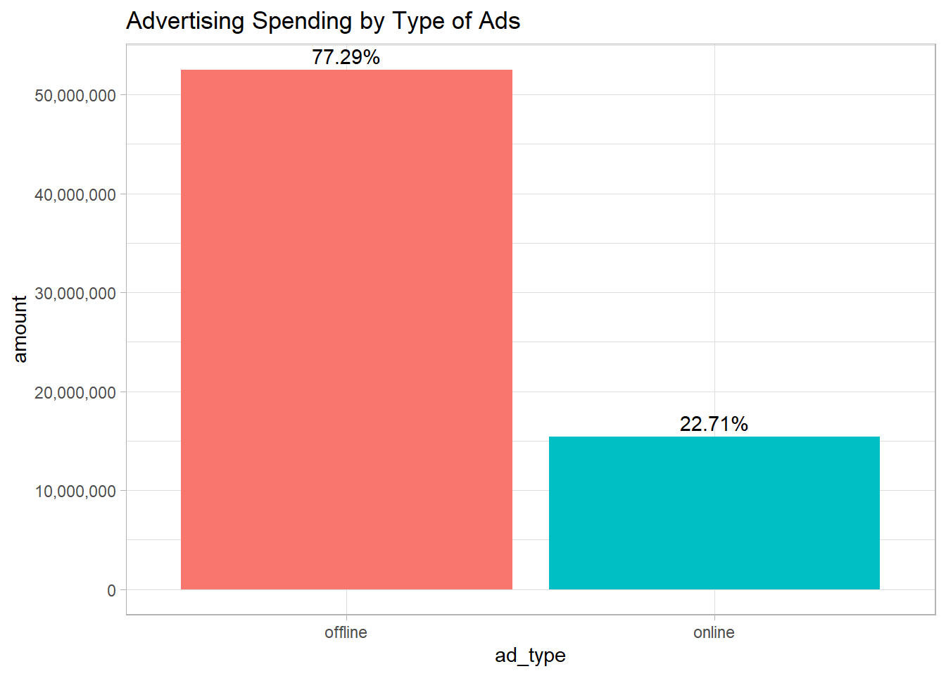

4 Marketing mix modeling

After exploring the main features of the data, we are ready to investigate the drivers of the web traffic performance. We will develop a multiple regression model that uses the traffic data as dependent variable (i.e. response variable) while Google AdWords, Facebook, TV, and radio variables will be used as independent variables, also known as predictors.

4.1 Modeling Diminishing Returns

At this point, an important decision we need to make is which functional form to use in the model. Shall we assume a linear or a non-linear relationship? Marketing literature suggests that the relationship between advertising and performance variables mostly follows a diminishing return pattern (Hanssens et al., 2001, 2014), as illustrated in the following plot.

This plot tells us that initially spending more and more money on advertising is beneficial but after a certain point the additional value gained from an extra spending will be very small. How can we introduce this type of non-linearity in the model? A typical approach is to use a log-log model specification. The log-log regression model suggests that log transformation is performed for both sides of the equation.

4.2 log-transformation

To estimate the model, we will perform log transformation on our variables.

Code

data <- data |> 
  mutate(lngoogle_adwords = log(google_adwords+1),
         lnfacebook = log(facebook+1),
         lntv = log(tv+1),
         lnradio = log(radio+1),
         lntraffic = log(traffic+1)
         )

The reason for adding +1 to the variables is that some variables include zero observations. When we take the logarithm of zero, it is not identified. Therefore, we should add a small number to be able to take the logarithm.

Code

#Creating Lagged Traffic Variable 
m <- 1   # one lag 

#number of observations
n <- length(data$traffic)

#Build Lag
data$L1.lntraffic <- c(rep(NA,m), data$lntraffic[1:(n-m)]) # --> c(NA, lntraffic[1:56])
data

week_beg	google_adwords	facebook	tv	radio	traffic	sum_online	sum_offline	lngoogle_adwords	lnfacebook	lntv	lnradio	lntraffic	L1.lntraffic
2020-07-06	94017.2	82950	0	0	6719812	176967.2	0	11.45124	11.32601	0.00000	0.00000	15.72057	NA
2020-07-13	93634.5	66150	0	0	6186229	159784.5	0	11.44716	11.09970	0.00000	0.00000	15.63784	15.72057
2020-07-20	112239.4	94650	0	0	6790416	206889.4	0	11.62840	11.45795	0.00000	0.00000	15.73102	15.63784
2020-07-27	121250.3	96450	0	0	7146957	217700.3	0	11.70562	11.47679	0.00000	0.00000	15.78220	15.73102
2020-08-03	130470.9	114600	0	0	7815741	245070.9	0	11.77891	11.64921	0.00000	0.00000	15.87165	15.78220
2020-08-10	131955.3	119550	0	0	8444791	251505.3	0	11.79023	11.69150	0.00000	0.00000	15.94906	15.87165
2020-08-17	129812.0	106350	0	0	8267982	236162.0	0	11.77385	11.57450	0.00000	0.00000	15.92790	15.94906
2020-08-24	110176.6	116550	0	0	7059093	226726.6	0	11.60985	11.66608	0.00000	0.00000	15.76983	15.92790
2020-08-31	97206.0	90150	0	1298507	6137780	187356.0	1298507	11.48460	11.40924	0.00000	14.07673	15.62997	15.76983
2020-09-07	107410.0	82650	0	0	6356676	190060.0	0	11.58442	11.32238	0.00000	0.00000	15.66502	15.62997
2020-09-14	77073.5	70650	0	0	5237124	147723.5	0	11.25253	11.16551	0.00000	0.00000	15.47128	15.66502
2020-09-21	103647.3	70950	0	0	4999990	174597.3	0	11.54876	11.16974	0.00000	0.00000	15.42495	15.47128
2020-09-28	116805.4	76650	0	0	5449003	193455.4	0	11.66827	11.24702	0.00000	0.00000	15.51094	15.42495
2020-10-05	148509.5	96750	0	0	6726743	245259.5	0	11.90841	11.47990	0.00000	0.00000	15.72160	15.51094
2020-10-12	125055.1	88500	4341824	0	6226920	213555.1	4341824	11.73652	11.39077	15.28381	0.00000	15.64439	15.72160
2020-10-19	142059.0	85650	0	0	6316911	227709.0	0	11.86400	11.35804	0.00000	0.00000	15.65874	15.64439
2020-10-26	137317.6	80400	0	0	6045622	217717.6	0	11.83006	11.29478	0.00000	0.00000	15.61485	15.65874
2020-11-02	169948.5	92250	0	0	6532776	262198.5	0	12.04326	11.43227	0.00000	0.00000	15.69234	15.61485
2020-11-09	180195.8	100500	0	0	7013419	280695.8	0	12.10180	11.51792	0.00000	0.00000	15.76334	15.69234
2020-11-16	171117.0	80400	0	0	6661626	251517.0	0	12.05011	11.29478	0.00000	0.00000	15.71187	15.76334
2020-11-23	322622.5	338700	6693444	1514925	13174892	661322.5	8208369	12.68424	12.73287	15.71664	14.23088	16.39382	15.71187
2020-11-30	212631.2	98100	4341824	0	7408386	310731.2	4341824	12.26732	11.49375	15.28381	0.00000	15.81812	16.39382
2020-12-07	234100.7	101400	4341824	1514925	8927318	335500.7	5856749	12.36351	11.52684	15.28381	14.23088	16.00463	15.81812
2020-12-14	260568.5	128850	4341824	0	10791803	389418.5	4341824	12.47062	11.76641	15.28381	0.00000	16.19430	16.00463
2020-12-21	290988.0	137250	4341824	1514925	12784412	428238.0	5856749	12.58104	11.82957	15.28381	14.23088	16.36374	16.19430
2020-12-28	133238.1	102600	0	0	8615943	235838.1	0	11.79990	11.53860	0.00000	0.00000	15.96913	16.36374
2021-01-04	109836.6	82350	0	0	4922788	192186.6	0	11.60676	11.31875	0.00000	0.00000	15.40939	15.96913
2021-01-11	128108.2	72900	0	0	4336508	201008.2	0	11.76064	11.19686	0.00000	0.00000	15.28258	15.40939
2021-01-18	119720.6	69750	0	0	4409387	189470.6	0	11.69292	11.15269	0.00000	0.00000	15.29925	15.28258
2021-01-25	128990.1	66000	0	0	4183630	194990.1	0	11.76750	11.09743	0.00000	0.00000	15.24669	15.29925
2021-02-01	135977.3	53700	0	0	3995216	189677.3	0	11.82025	10.89119	0.00000	0.00000	15.20061	15.24669
2021-02-08	143930.6	131400	0	0	4505004	275330.6	0	11.87709	11.78601	0.00000	0.00000	15.32070	15.20061
2021-02-15	145172.9	73800	0	0	5002462	218972.9	0	11.88569	11.20913	0.00000	0.00000	15.42544	15.32070
2021-02-22	168285.3	85050	0	0	5252341	253335.3	0	12.03342	11.35101	0.00000	0.00000	15.47418	15.42544
2021-03-01	176839.9	81450	0	0	5112821	258289.9	0	12.08301	11.30776	0.00000	0.00000	15.44726	15.47418
2021-03-08	189027.1	85050	4397123	1511474	5689169	274077.1	5908598	12.14965	11.35101	15.29646	14.22860	15.55407	15.44726
2021-03-15	180690.1	101250	0	0	6502390	281940.1	0	12.10454	11.52536	0.00000	0.00000	15.68768	15.55407
2021-03-22	171390.5	76200	0	0	5524652	247590.5	0	12.05171	11.24113	0.00000	0.00000	15.52473	15.68768
2021-03-29	162937.5	83550	0	0	5214240	246487.5	0	12.00113	11.33321	0.00000	0.00000	15.46690	15.52473
2021-04-05	177504.1	90450	0	0	5687588	267954.1	0	12.08675	11.41256	0.00000	0.00000	15.55380	15.46690
2021-04-12	193782.7	104100	0	0	5847569	297882.7	0	12.17450	11.55312	0.00000	0.00000	15.58154	15.55380
2021-04-19	209021.0	111000	4397123	1511474	7508050	320021.0	5908598	12.25019	11.61729	15.29646	14.22860	15.83149	15.58154
2021-04-26	144461.4	90000	0	0	5374538	234461.4	0	11.88077	11.40758	0.00000	0.00000	15.49718	15.83149
2021-05-03	124752.6	73800	0	0	4588852	198552.6	0	11.73410	11.20913	0.00000	0.00000	15.33914	15.49718
2021-05-10	169455.0	115050	0	0	5512025	284505.0	0	12.04035	11.65313	0.00000	0.00000	15.52244	15.33914
2021-05-17	190908.2	376650	0	0	6834931	567558.2	0	12.15955	12.83907	0.00000	0.00000	15.73756	15.52244
2021-05-24	185839.3	144900	0	0	6863975	330739.3	0	12.13264	11.88381	0.00000	0.00000	15.74180	15.73756
2021-05-31	180518.6	290850	0	0	7158438	471368.6	0	12.10359	12.58057	0.00000	0.00000	15.78380	15.74180
2021-06-07	193529.5	139350	4397123	0	7074652	332879.5	4397123	12.17319	11.84475	15.29646	0.00000	15.77203	15.78380
2021-06-14	147352.4	116250	0	0	6488603	263602.4	0	11.90059	11.66351	0.00000	0.00000	15.68556	15.77203
2021-06-21	148203.4	131850	0	0	6464867	280053.4	0	11.90635	11.78943	0.00000	0.00000	15.68189	15.68556
2021-06-28	159418.6	126750	0	0	7041649	286168.6	0	11.97929	11.74998	0.00000	0.00000	15.76735	15.68189
2021-07-05	154105.7	147150	0	1036439	6832453	301255.7	1036439	11.94540	11.89921	0.00000	13.85130	15.73719	15.76735
2021-07-12	132009.8	106200	0	0	5883640	238209.8	0	11.79064	11.57309	0.00000	0.00000	15.58769	15.73719
2021-07-19	183341.3	214500	0	0	5900047	397841.3	0	12.11911	12.27607	0.00000	0.00000	15.59047	15.58769
2021-07-26	189316.0	133200	0	1036439	6549324	322516.0	1036439	12.15118	11.79961	0.00000	13.85130	15.69487	15.59047
2021-08-02	201080.7	142950	0	0	7018006	344030.7	0	12.21147	11.87026	0.00000	0.00000	15.76399	15.69487

Code

#Fit a Regression 
options(scipen=999)
#options(scipen = 0)

modfit <- lm(lntraffic ~ L1.lntraffic + lngoogle_adwords + lnfacebook + lntv + lnradio, data=data)
summary(modfit)


Call:
lm(formula = lntraffic ~ L1.lntraffic + lngoogle_adwords + lnfacebook + 
    lntv + lnradio, data = data)

Residuals:
     Min       1Q   Median       3Q      Max 
-0.32118 -0.08169 -0.00214  0.08718  0.21416 

Coefficients:
                 Estimate Std. Error t value      Pr(>|t|)    
(Intercept)      3.150739   1.498074   2.103       0.04050 *  
L1.lntraffic     0.535935   0.076474   7.008 0.00000000583 ***
lngoogle_adwords 0.155433   0.089834   1.730       0.08976 .  
lnfacebook       0.193668   0.056041   3.456       0.00113 ** 
lntv             0.004569   0.004282   1.067       0.29107    
lnradio          0.006963   0.004046   1.721       0.09147 .  
---
Signif. codes:  0 '***' 0.001 '**' 0.01 '*' 0.05 '.' 0.1 ' ' 1

Residual standard error: 0.1252 on 50 degrees of freedom
  (1 observation deleted due to missingness)
Multiple R-squared:  0.7578,    Adjusted R-squared:  0.7336 
F-statistic: 31.29 on 5 and 50 DF,  p-value: 0.0000000000000273

Code

# tidyverse way
data %>% 
  lm(lntraffic ~ L1.lntraffic + lngoogle_adwords + lnfacebook + 
       lntv + lnradio, data=.) %>% 
  summary()


Call:
lm(formula = lntraffic ~ L1.lntraffic + lngoogle_adwords + lnfacebook + 
    lntv + lnradio, data = .)

Residuals:
     Min       1Q   Median       3Q      Max 
-0.32118 -0.08169 -0.00214  0.08718  0.21416 

Coefficients:
                 Estimate Std. Error t value      Pr(>|t|)    
(Intercept)      3.150739   1.498074   2.103       0.04050 *  
L1.lntraffic     0.535935   0.076474   7.008 0.00000000583 ***
lngoogle_adwords 0.155433   0.089834   1.730       0.08976 .  
lnfacebook       0.193668   0.056041   3.456       0.00113 ** 
lntv             0.004569   0.004282   1.067       0.29107    
lnradio          0.006963   0.004046   1.721       0.09147 .  
---
Signif. codes:  0 '***' 0.001 '**' 0.01 '*' 0.05 '.' 0.1 ' ' 1

Residual standard error: 0.1252 on 50 degrees of freedom
  (1 observation deleted due to missingness)
Multiple R-squared:  0.7578,    Adjusted R-squared:  0.7336 
F-statistic: 31.29 on 5 and 50 DF,  p-value: 0.0000000000000273

4.3 Model Output

Residuals:

Residuals represent the ‘unexplained’ part of the model, i.e. the impact of other factors that are not explicitly included in the model. The descriptive statistics (e.g. min, max) of residuals are reported at the top of the model output.

Coefficient estimates:

We can write down the estimated coefficients of this marketing mix model in an equation format:

The standard error of each coefficient shows at what precision level we estimated that particular coefficient, i.e. represents the uncertainty surrounding that coefficient. The t-value is obtained by dividing the coefficient by its standard error. P-value, Pr(>|t|), is computed based on the t-value, and helps us understand whether the coefficient is statistically significant. For example, lagged traffic is a strong indicator of the next period’s traffic as it is highly significant (p-value is close to zero). The effect of Facebook ads is significant at 1% level while Google AdWords and Radio effects are significant at 10% level. Finally, the effect of TV ads is not statistically significant.

4.4 Model Fit

After we estimate the coefficients, we can obtain the model fit plot to see whether our model captures the patterns in the traffic data.

line plot

Code

# Model fit plot 
fitted_traffic <- ts(modfit$fitted.values, frequency = 52, start=c(2020,28))
fitted_traffic <- c(NA, fitted_traffic)

plot(data$lntraffic, type="l", col="blue", main="Web Traffic",lwd=3)# l=line, lwd=line width
lines(fitted_traffic, type="b", col="red") # b=both
legend("topleft", lty=1, col=c("blue", "red"), #lty=line type; 1=solid line, 2=dotted line
       c("Logged Traffic Data","Fitted"))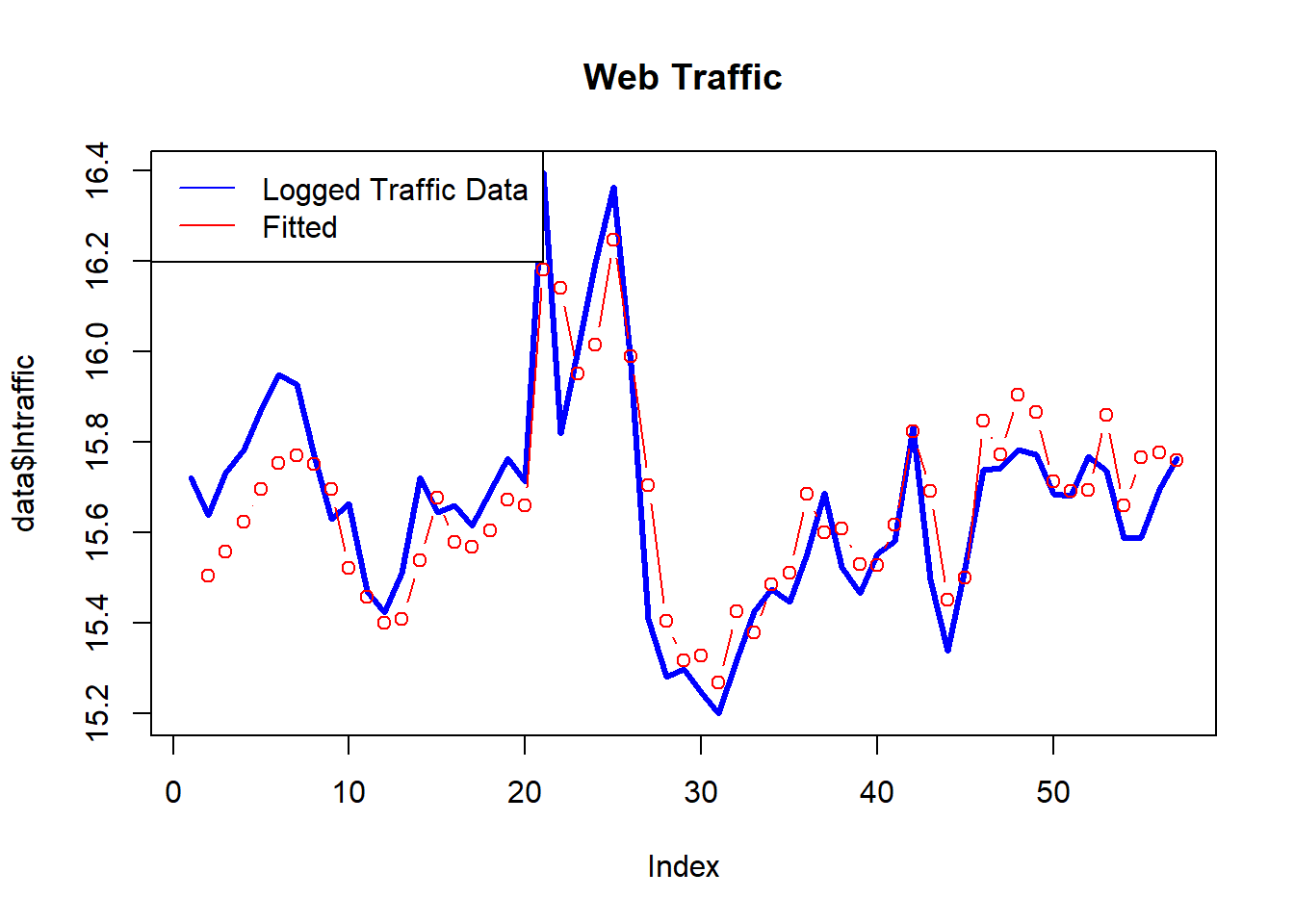

line plot

Code

data <- data.frame(data, fitted_traffic)

data |> 
  pivot_longer(c(lntraffic,fitted_traffic), 
               names_to = "type", values_to = "value") |> 
  ggplot(aes(week_beg, value, color = type)) +
  geom_line() +
  labs(title = "How does fitted traffic capture actual traffic?",
       x = "Begining of Week",
       color = "")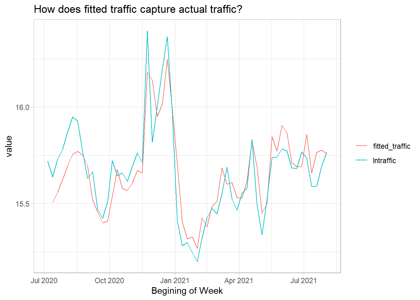

4.5 Model Diagnostics

Once we estimate our marketing mix model, it is usually a good practice to perform model diagnostic checks on the estimated residuals. In the marketing mix model above, we assume that residuals are uncorrelated (i.e.independent), have zero mean and constant variance. If the model passes these diagnostics, we conclude that the model is not misspecified and can be used to make statistical inferences and predictions.

Core Assumptions of Linear Regression

Assumption	Diagnostic Test / Plot	Explanation
Linearity	Residuals vs Fitted Plot	Residuals should have no pattern (random scatter).
Independence of errors	Durbin-Watson Test, ACF Plot	Especially important in time series data.
Homoscedasticity (constant variance)	Scale-Location Plot, Residuals vs Fitted Plot	Variance of residuals should be constant across fitted values.
Normality of residuals	Q-Q Plot, Histogram of residuals	Needed for valid hypothesis tests and confidence intervals.
No multicollinearity	Variance Inflation Factor (VIF)	Predictors should not be highly correlated.
No influential outliers	Cook’s Distance, Standardized Residuals	Outliers can disproportionately influence the regression line.

Next, we turn our attention to the following questions that are central to the case study:

What drives the web traffic performance?
What is the traffic return on marketing investment?
What is the optimal budget allocation?

5 What drives web traffic performance?

What is the marketing’s contribution to web traffic performance? How much traffic was generated thanks to Google AdWords, Facebook, TV, and radio? To see this, first, we need to convert the elasticities to unit effects using the following formula:

5.1 Calculating unit effects

The following code chunk retrieves the coefficients (elasticities) from our log-log model output and then computes the unit effects.

Code

#Retrieve each model coefficient: 
beta_adwords <- summary(modfit)$coefficients[3,1]
beta_facebook <- summary(modfit)$coefficients[4,1]
beta_tv <- summary(modfit)$coefficients[5,1]
beta_radio <- summary(modfit)$coefficients[6,1]

#Calculate the baseline (average) traffic: 
average_traffic <- mean(traffic)

#Calculate the baseline (average) advertising spending for each media: 
average_adwords <- mean(google_adwords)
average_facebook <- mean(facebook)
average_tv <- mean(tv)
average_radio <- mean(radio)

# Finally, calculate the unit effects: 
theta_adwords <- beta_adwords*(average_traffic/average_adwords)
theta_facebook <- beta_facebook*(average_traffic/average_facebook)
theta_tv <- beta_tv*(average_traffic/average_tv)
theta_radio <- beta_radio*(average_traffic/average_radio)

5.2 Calculating media contribution

Next, we compute the contribution of each advertising media to the overall traffic performance using the following formula:

Code

#How much traffic we got thanks to TV, Adwords etc.?
sum_adwords <- sum(google_adwords)
sum_facebook <- sum(facebook)
sum_tv <- sum(tv)
sum_radio <- sum(radio)


#Each media's contribution to traffic 
adwords_contribution <- theta_adwords * sum_adwords
facebook_contribution <- theta_facebook * sum_facebook
tv_contribution <- theta_tv * sum_tv
radio_contribution <- theta_radio*sum_radio

print(adwords_contribution)

[1] 57994699

Code

print(facebook_contribution)

[1] 72261042

Code

print (tv_contribution)

[1] 1704751

Code

print (radio_contribution)

[1] 2597922

5.3 Visualizing media contributions

We need to plug in the necessary data for the bar plot. So, we need the following pieces:

Code

# Bar plot information 
media_contribution <- c(adwords_contribution,
                        facebook_contribution,
                        tv_contribution, 
                        radio_contribution)

media_contribution = round(media_contribution, digits=0)

media_names <- c("AdWords","Facebook", "TV","Radio")
df <- data.frame(media_names, media_contribution)
head(df)

media_names	media_contribution
AdWords	57994699
Facebook	72261042
TV	1704751
Radio	2597922

Cross-checking data

Code

data <- data |> 
  as_tibble() 

# total actual traffic 
data |> 
  summarize(total_traffic = sum(traffic))

total_traffic
373118180

Code

# total media contribution
sum(media_contribution)

[1] 134558414

Bar Plot with total

We will use this information to create a bar plot of the web traffic contribution of each media:

Code

df <- df |> as_tibble()
df |>   
  mutate(media_names = as_factor(media_names)) |> 
  mutate(media_names = fct_reorder(media_names, -media_contribution)) |> 
  ggplot(aes(media_names, media_contribution, fill = media_names)) +
  geom_col(show.legend = FALSE) +
  geom_text(aes(label=media_contribution), vjust=-0.3, size=3.5) +
  scale_y_continuous(labels = comma_format()) +
  labs(title="Contribution to Traffic", 
       x="Media", 
       y="Contribution") +
  theme_minimal()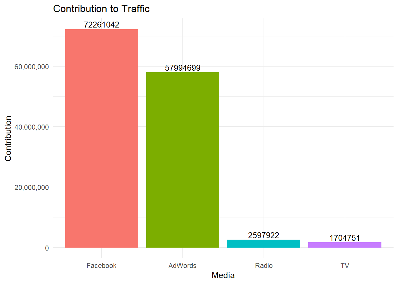

Bar Plot with Percentage

Sometimes, it is difficult to communicate large numbers displayed above the bars. To avoid this, we can compute the contribution of each traffic driver in percentage terms.

Code

#install.packages("viridis")
library(viridis)
df |> 
  mutate(percent_media_cont = media_contribution/sum(media_contribution)) |> 
  mutate(media_names = fct_reorder(media_names, percent_media_cont, .desc = TRUE)) |> 
  ggplot(aes(media_names, percent_media_cont)) + 
  geom_col(aes(fill=media_names), show.legend = FALSE) +
  geom_text(aes(label=paste0(round(percent_media_cont*100, digits = 2),"%")), 
            vjust=-0.3) +
  labs(title="Contribution to Traffic", 
       x="Media", 
       y="Contribution") +
  theme_minimal()+
  scale_y_continuous(labels = percent_format()) +
  scale_fill_viridis(discrete = TRUE)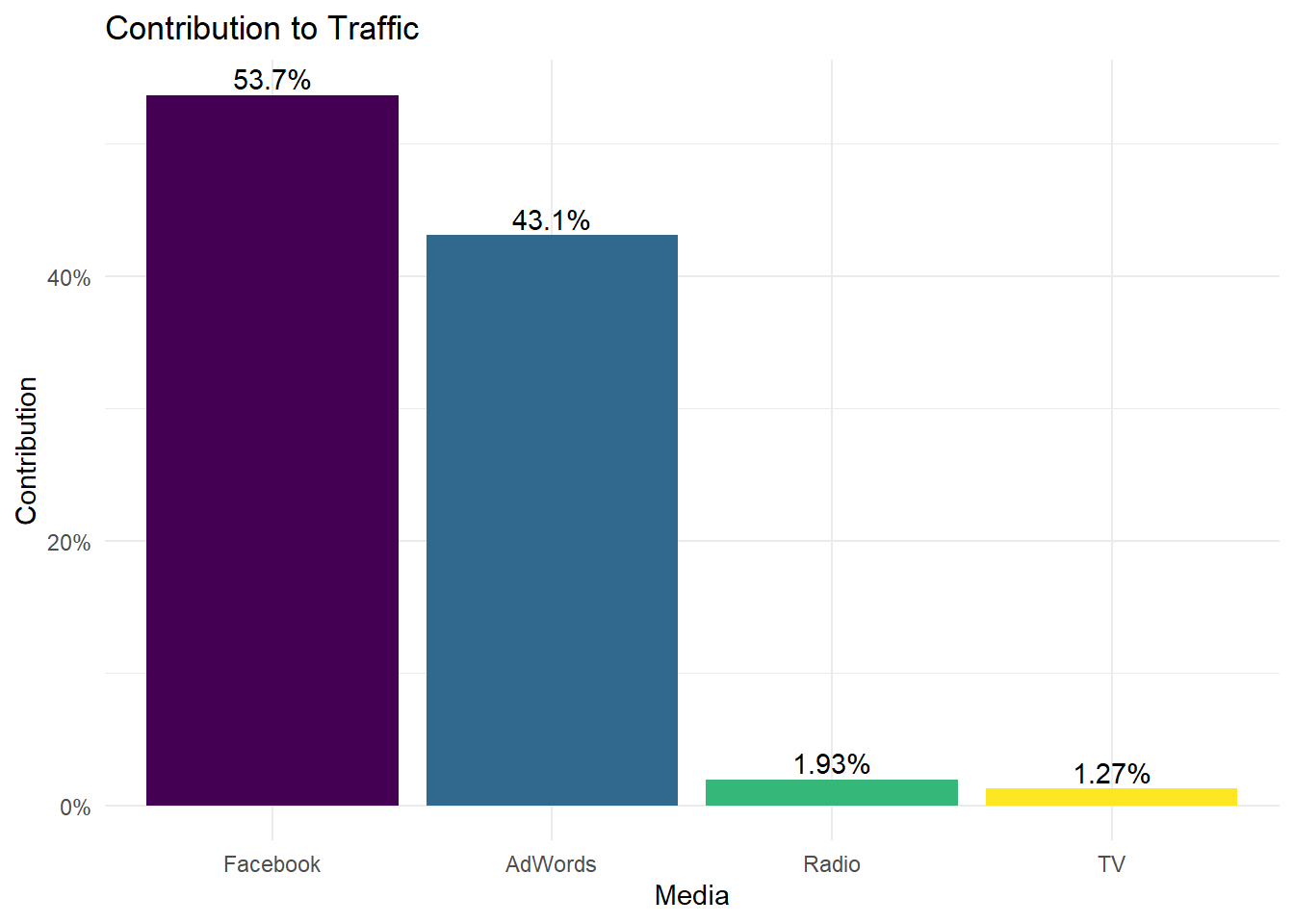

The bar plot above suggests that 53.7% of the web traffic is driven by Facebook, 43.1% is driven by Google AdWords, 1.9% by radio, and 1.3% by TV.

6 Return on Marketing Investment (ROMI)

Financially oriented marketing executives are very often concerned about the return on marketing investment (ROMI). That is, they would like to know how much they earn with respect to how much they spend. Usually, the return metric is sales, revenues, or profits. However, it can also be something non-financial, e.g.customer engagement, web traffic and store traffic.

Let’s calculate the traffic return on marketing investment (TROMI) for FourTex.

The first input we need is the cost data:

Code

#Calculate the cost of each media
cost_adwords <- sum(google_adwords)
cost_facebook <- sum(facebook)
cost_tv <- sum(tv)
cost_radio <- sum(radio)
cost_total <- cost_adwords+cost_facebook+cost_tv+cost_radio

# cross-checking
data |> 
  summarize(sum_adwords = sum(google_adwords))

sum_adwords
8999557

Code

data |> 
  summarize(total_spend = 
              sum(google_adwords) + sum(facebook) + sum(tv) + sum(radio))

total_spend
67969701

Code

# adding media cost vector to data
cost <- c(cost_adwords,cost_facebook,cost_tv,cost_radio)
cost = round(cost, digits=0)

df <- data.frame(df, cost)
df

media_names	media_contribution	cost
AdWords	57994699	8999557
Facebook	72261042	6437100
TV	1704751	41593933
Radio	2597922	10939111

6.1 Barplot with cost vs.traffic contribution (Dodged)

Then, we can see the traffic return and cost data together in a bar plot:

Code

df <- df |> 
  as_tibble() |> 
  rename(traffic = media_contribution) 

df |> 
  pivot_longer(-media_names, names_to = "traf_cost", values_to = "value") |> 
  mutate(media_names = fct_reorder(media_names, -value)) |> 
  ggplot(aes(media_names, value, fill = traf_cost)) +
  geom_col(position = position_dodge())+
  scale_y_continuous(labels = comma_format()) +
  labs(title = "Traffic vs. Media Cost",
       x = "Media",
       y = "Traffic and Cost")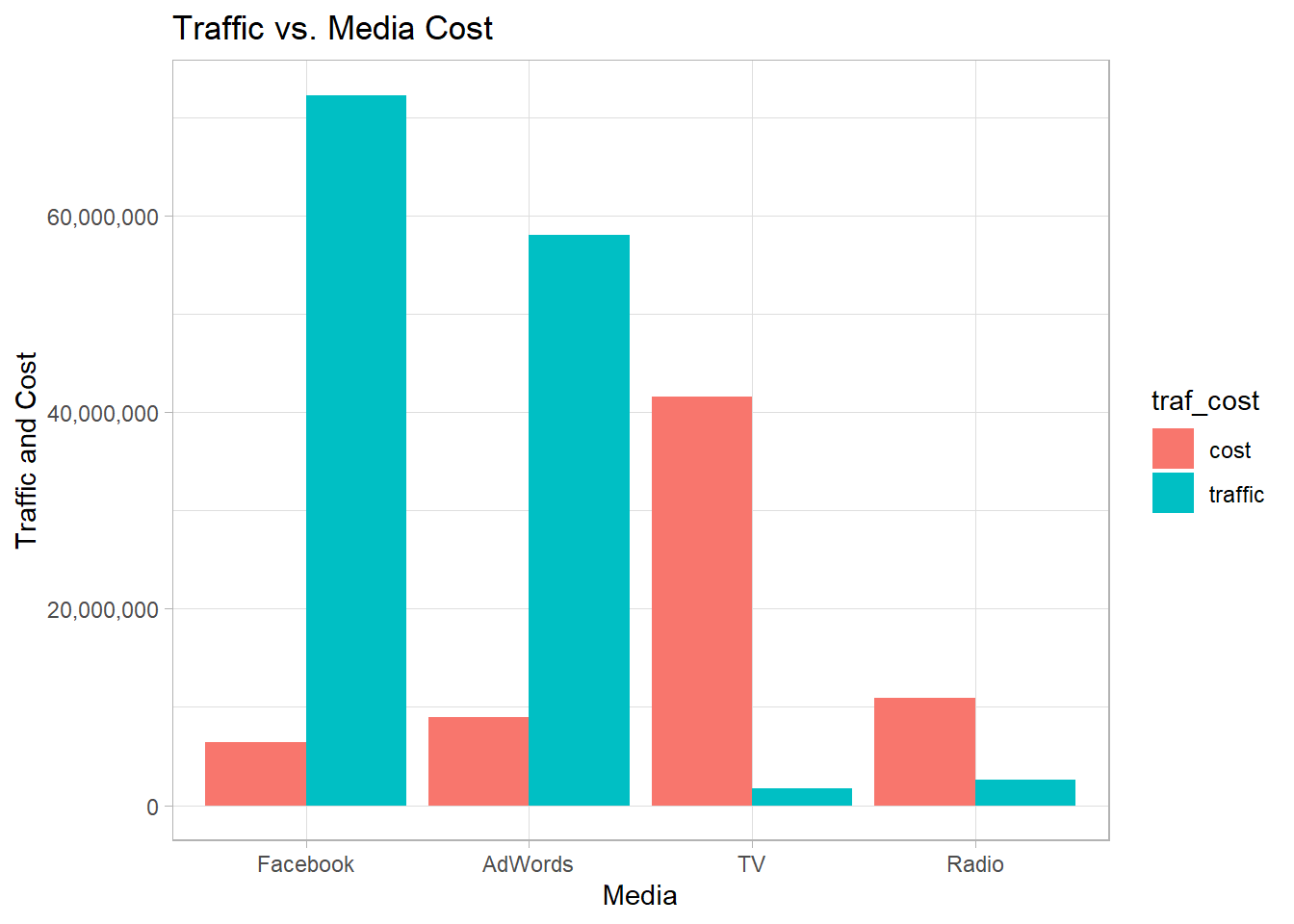

6.2 Barplot with TROMI

Instead of showing cost and return data together, we can just compute the TROMI, and show the results in percentages. To do so, we need to divide the traffic contribution of each media by the cost of each media:

Code

# Calculate the traffic return for each media 

df <- df |> 
  mutate(roi = round(traffic/cost, digits = 1))

Code

# data manipulation
df |> 
  mutate(media_names = fct_reorder(media_names, -roi)) |> 
  ggplot(aes(media_names, roi, fill = media_names)) +
  geom_col(show.legend = FALSE)+
  geom_text(aes(label=roi), vjust=-0.3, size=3.5) +
  scale_fill_viridis(discrete = TRUE) +
  labs(title="Traffic Return on Marketing Investment", 
       x="Media", 
       y="TROMI") +
  theme_bw()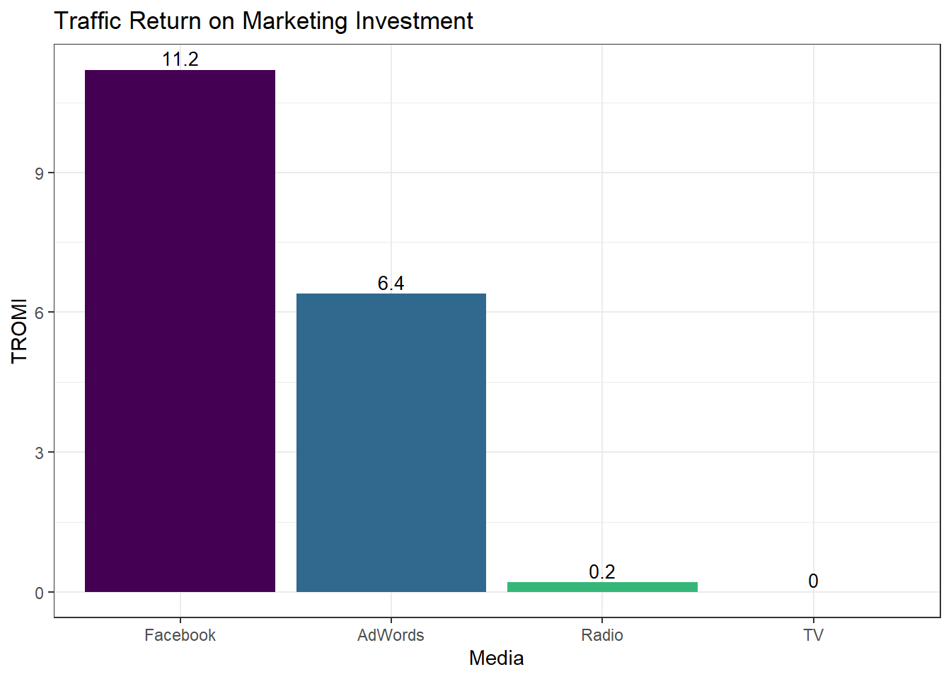

7 Marketing budget allocation

Marketing analysts follow two main approaches to guide their resource allocation strategies. One of them is normative decision making based on constrained optimization models (e.g.profit maximization subject to budget constraints).

Another method is elasticity-based allocation. In this R application, we will allocate the marketing budget of FourTex by making use of the elasticities obtained from the log-log regression model.

7.1 Actual budget spending

Before diving into the optimal resource allocation, let’s see what the current budget allocation looks like:

Pie Chart

Code

df <- df |> 
  mutate(costshare = cost/sum(cost))

#library(ggrepel)
df |> 
  ggplot(aes(x="", y = costshare, fill = media_names))+
  geom_bar(stat = "identity", width = 1)+
  coord_polar("y", start = 0) +
  geom_text(aes(label = paste0(round(costshare*100, digits = 1),"%")),
            position = position_stack(vjust = 0.2),
            hjust = 0.2)+
  geom_label(aes(label = media_names),
             position = position_stack(vjust = 0.8),
             hjust = 0.7,
             show.legend = FALSE) +
  labs(title = "Actual Ad Spending",
       x = "",
       y = "") +
  theme_void() +
  theme(legend.position = "none")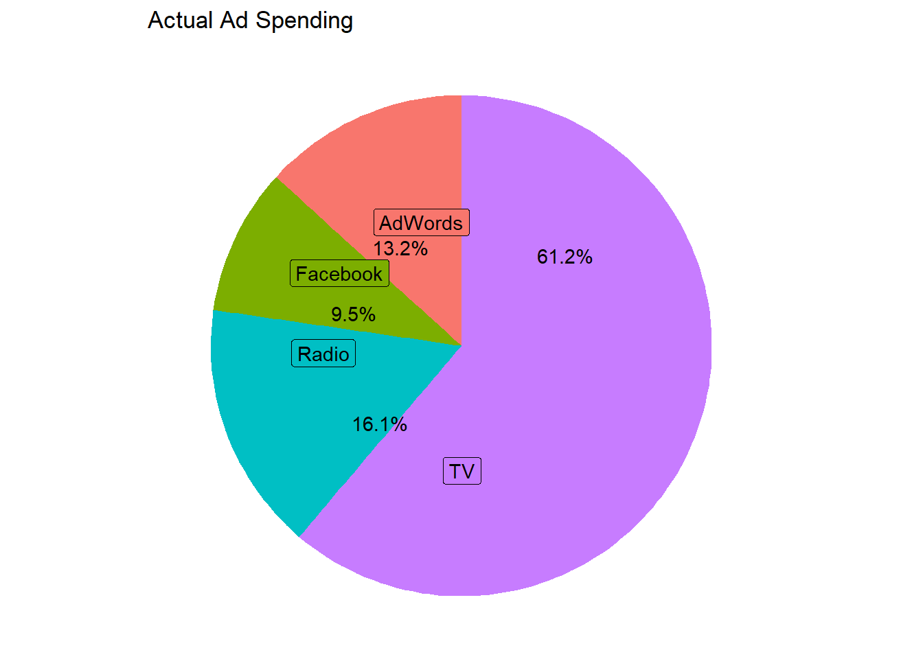

7.2 Elasticity-Based Allocation

Pie chart with Base R

Code

#The sum of all elasticities 
beta_allmedia <- beta_adwords + beta_facebook + beta_tv + beta_radio

#Optimal resource allocation
optim_adwords <- beta_adwords/beta_allmedia
optim_facebook <- beta_facebook/beta_allmedia
optim_tv <- beta_tv/beta_allmedia
optim_radio <- beta_radio/beta_allmedia

You can see the computed allocation at the top right of the screen under the Environment tab. Now, we can get a pie-chart that shows the allocation visually with percentages.

Code

## Pie-chart ingredients 
optimal_spend <- c(optim_adwords,optim_facebook,optim_tv,optim_radio)
optimal_spend = round(optimal_spend, digits=2)
optimal_spend

[1] 0.43 0.54 0.01 0.02

Code

slices_optim <- c(optim_adwords,optim_facebook,optim_tv,optim_radio)
lbls_optim <- c("Adwords", "Facebook", "TV","Radio")
pct_optim <- round(slices_optim*100)
lbls_optim <- paste(lbls_optim, pct_optim) # paste variable names to data labels 
lbls_optim <- paste(lbls_optim, "%", sep="") # add % sign to labels

# Get the pie-chart
pie(slices_optim, labels=lbls_optim, col=rainbow(length(lbls_optim)), main="Optimal Budget Allocation" )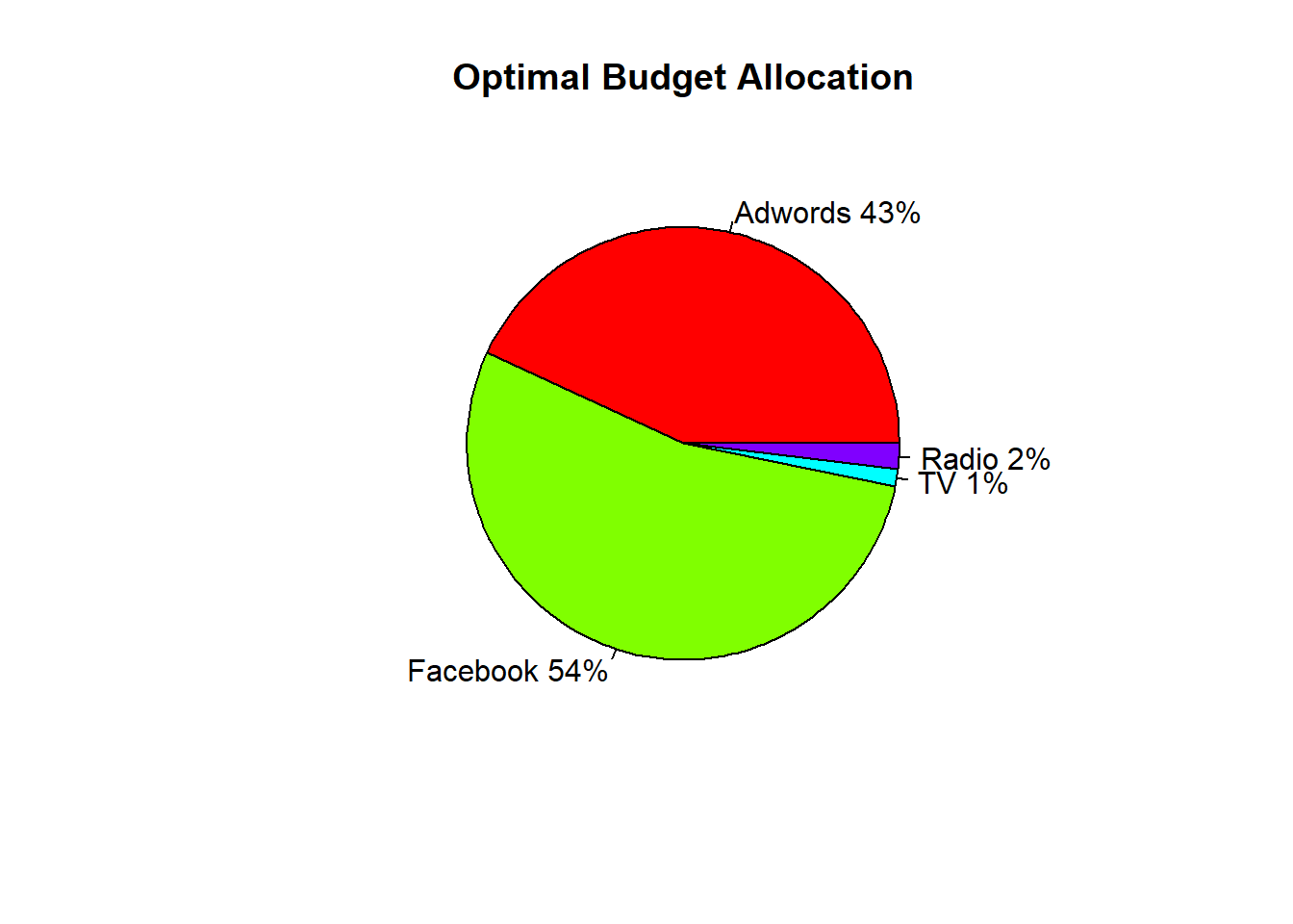

Pie chart with tidyverse

Code

# Create a vector
beta <- c(beta_adwords, beta_facebook, beta_tv, beta_radio)

# additing it to df
df <- data.frame(df, beta)

# creating percentage
df <- df |> 
  mutate(opt_alloca = beta/sum(beta))
df

media_names	traffic	cost	roi	costshare	beta	opt_alloca
AdWords	57994699	8999557	6.4	0.1324054	0.1554325	0.4310002
Facebook	72261042	6437100	11.2	0.0947054	0.1936680	0.5370236
TV	1704751	41593933	0.0	0.6119482	0.0045689	0.0126692
Radio	2597922	10939111	0.2	0.1609410	0.0069627	0.0193070

Code

# chart
df |> 
  ggplot(aes(x="", y = opt_alloca, fill = media_names))+
  geom_bar(stat = "identity", width = 1)+
  coord_polar("y", start = 0) +
  geom_text(aes(label = paste0(round(opt_alloca*100, digits = 1),"%")),
            position = position_stack(vjust = 0.7),
            hjust = 0.9) +
  geom_label(aes(label = media_names),
             position = position_stack(vjust = 0.2),
             hjust = 0.3,
             show.legend = FALSE) +
  labs(title = "Optimal Budget Allocation",
       x = "",
       y = "") +
  theme_void() +
  theme(legend.position = "right")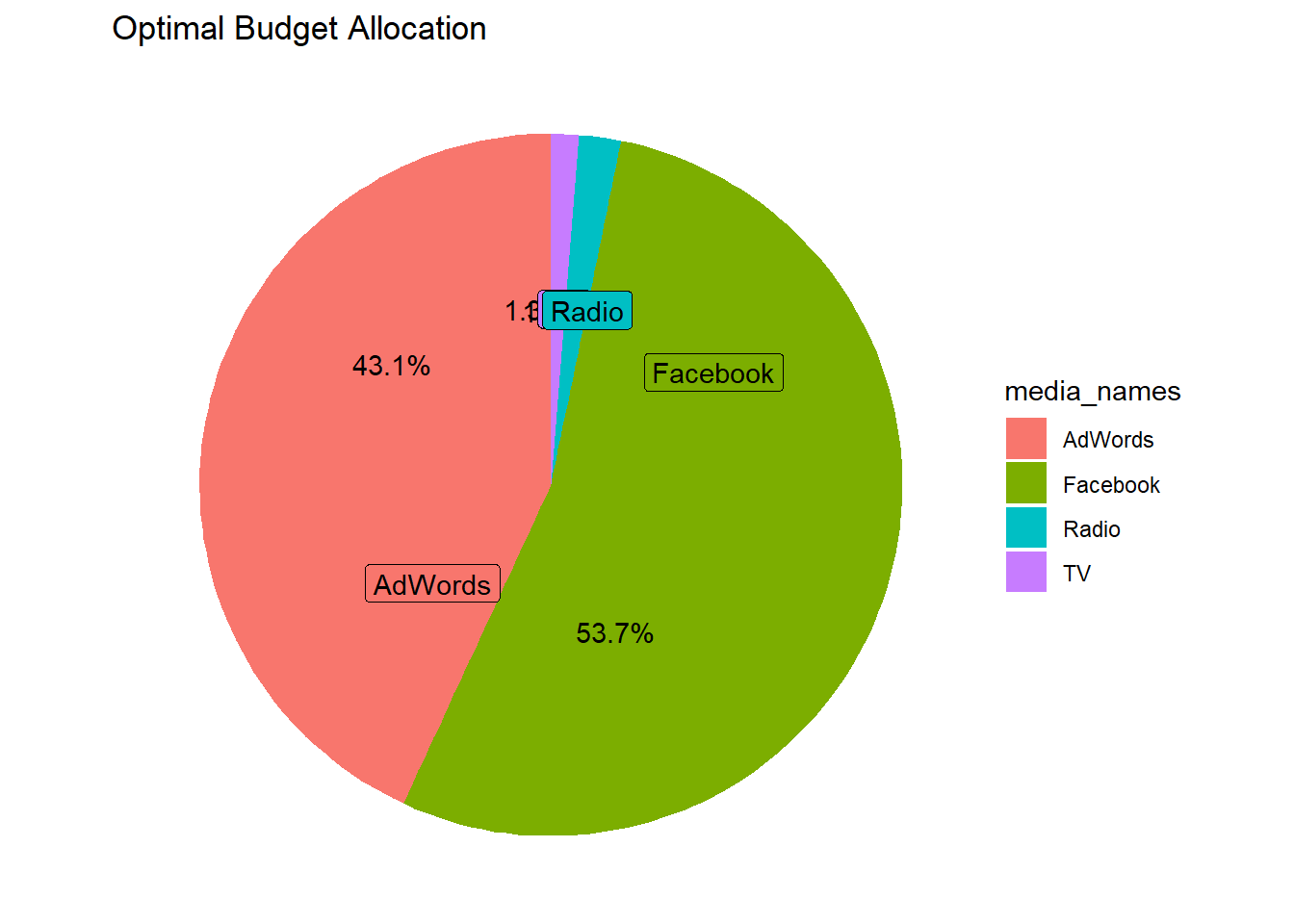

8 Results

The FourTex case study shows a clear imbalance between where marketing budget is spent and which channels actually drive website traffic. Based on the model results, digital channels are the strongest contributors to web traffic, while offline media delivers little measurable impact in this traffic-focused framework.

More specifically, Facebook is the most effective channel, with an estimated elasticity of 0.194, meaning that a 10% increase in Facebook spend is associated with a 1.94% increase in web traffic.

Google also performs strongly, with an elasticity of 0.155, or roughly a 1.55% traffic increase for every 10% increase in spend.

In contrast, radio has only a 0.007 elasticity, and TV just 0.005, indicating very limited responsiveness. These weak offline effects are also less reliable statistically: Facebook is highly significant (p = 0.00113), radio is only marginally significant (p = 0.09147), and TV is not statistically significant (p = 0.29107).

The model also confirms that traffic is not driven by advertising alone. The inclusion of the lagged traffic term is important, as its coefficient of 0.536 suggests that around 54% of traffic momentum carries over into the following period. This indicates that website visits are partly persistent over time, and that current performance reflects both present marketing activity and past traffic dynamics.

In terms of model quality, the results are reasonably strong. The regression explains about 75.8% of the variation in website traffic (R² = 0.7578), with an adjusted R² of 0.7336, which suggests the model captures substantial variation without severe overfitting. In addition, the residual standard error of 0.1252 indicates that prediction error remains relatively modest for a log-log specification. Taken together, these figures suggest the model provides a credible basis for managerial interpretation.

From a return-on-investment perspective, the contrast across channels is even more striking. Facebook generates 11.2 visits per £1 spent, making it the most efficient channel in the mix. Google returns 6.4 visits per £1 spent, also making it a strong performer. By comparison, radio returns only 0.2 visits per £1 spent, while TV generates effectively 0 visits per £1 spent in this model. Despite these results, FourTex currently allocates 77% of its budget to offline media and only 23% to online channels, even though digital activity accounts for approximately 97% of attributed website traffic.

These findings suggest that the current allocation is poorly aligned with the objective of maximizing web traffic. If traffic generation is the primary goal, FourTex should substantially reduce investment in TV and radio and reallocate budget toward Facebook and Google. The optimization results support this conclusion, indicating that the budget should be directed almost entirely toward the two digital channels, which together account for the overwhelming majority of measurable traffic response.

At the same time, the weak returns from TV and radio should be interpreted carefully. A traffic model captures direct and relatively immediate website response, but offline media often works through brand awareness, delayed effects, and assisted pathways that are harder to observe in session-level traffic data. This means that TV and radio may still have strategic value, but not necessarily for the specific outcome measured here. If FourTex wants to justify continued offline investment, those channels should be evaluated against broader KPIs such as sales, brand lift, or long-term customer acquisition, rather than web traffic alone.

Code

library(gt)
library(scales)

df %>%
  mutate(
    media_names = factor(media_names, levels = media_names)
  ) %>%
  gt() %>%
  tab_header(
    title = md("**Marketing Mix Model Summary**")
  ) %>%
  cols_label(
    media_names = "Channel",
    traffic = "Attributed Traffic",
    cost = "Cost",
    roi = "ROI",
    costshare = "Cost Share",
    beta = "Beta",
    opt_alloca = "Optimal Allocation"
  ) %>%
  fmt_number(columns = c(traffic, cost), decimals = 0, sep_mark = ",") %>%
  fmt_number(columns = c(roi, beta), decimals = 2) %>%
  fmt_percent(columns = c(costshare, opt_alloca), decimals = 1) %>%
  cols_align(align = "center", columns = everything()) %>%
  tab_options(
    table.font.size = px(13),
    data_row.padding = px(6)
  )

Channel	Attributed Traffic	Cost	ROI	Cost Share	Beta	Optimal Allocation
Marketing Mix Model Summary
AdWords	57,994,699	8,999,557	6.40	13.2%	0.16	43.1%
Facebook	72,261,042	6,437,100	11.20	9.5%	0.19	53.7%
TV	1,704,751	41,593,933	0.00	61.2%	0.00	1.3%
Radio	2,597,922	10,939,111	0.20	16.1%	0.01	1.9%

Metric meanings

Attributed Traffic: estimated traffic generated by each media channel in the model.
Cost: total spend for that channel.
ROI: return on investment, usually interpreted as traffic or return generated per unit of spend.
Cost Share: proportion of the total budget currently spent on that channel.
Beta: regression coefficient from the MMM; it shows the direction and strength of the channel’s relationship with traffic, holding other variables constant.
Optimal Allocation: recommended share of total budget to assign to that channel based on the optimization output.

9 Conclusion

Overall, the central conclusion is that Facebook and Google are the true performance drivers for website traffic, while TV and radio show minimal direct contribution in this model. For a traffic objective, FourTex should rebalance its spending toward digital media, where both elasticities and returns on marketing investment are substantially higher. However, if the company’s goal shifts from traffic to another metric such as sales or brand growth, the optimal allocation could look very different. In that sense, the most important managerial lesson is that marketing mix decisions should always be aligned with the specific business outcome being optimized.