Post-Campaign Sales Analysis with Differences-in-Differences

causal inference
exploratory data analysis
Differences-in-Differences method is used to estimate the causal effect of a marketing campaign on sales.
Author

Ceren Unal

In retail environments, randomized A/B testing is often impractical when evaluating marketing campaigns. Store selection for promotional initiatives may be driven by regional strategies, franchise agreements, or operational constraints rather than random assignment. Additionally, withholding potentially revenue-generating campaigns from stores purely for experimental purposes raises ethical and business concerns.

This analysis evaluates a sales campaign implemented across 30 treatment stores using a difference-in-differences (DiD) approach. By comparing sales trends in treatment stores against 30 control stores over an 8-week period (4 weeks pre-campaign, 4 weeks post-campaign), we can isolate the campaign’s causal effect. The DiD method accounts for baseline differences between stores and common time trends, measuring whether treatment stores experienced different sales growth compared to what would have occurred absent the intervention, captured by the control group’s trajectory.

1 Load Packages & Data

We’ll be using Tidyverse and base R to prepare our dataset and run a linear regression model.

Code
library(tidyverse)  # ggplot(), %>%, mutate(), and friends
library(scales)  # Format numbers with functions like comma(), percent(), and dollar()

sales <- read.csv("did_store_sales.csv")

glimpse(sales)
Rows: 480
Columns: 5
$ store_id <chr> "T01", "T01", "T01", "T01", "T01", "T01", "T01", "T01", "T02"…
$ group    <chr> "Treatment", "Treatment", "Treatment", "Treatment", "Treatmen…
$ week     <int> 1, 2, 3, 4, 5, 6, 7, 8, 1, 2, 3, 4, 5, 6, 7, 8, 1, 2, 3, 4, 5…
$ period   <chr> "Pre", "Pre", "Pre", "Pre", "Post", "Post", "Post", "Post", "…
$ sales    <dbl> 25105.73, 25167.54, 22865.04, 26339.08, 29417.32, 30581.67, 3…

2 Exploratory Data Analysis

We have 480 observations across 60 stores. The observations are divided into “Pre” and “Post” treatment periods as indicated in the period variable. The stores are divided into “Treatment” and “Control” groups and identified as such in the group variable. The revenue recorded for each observation is stored in the sales variable.

Code
skimr::skim(sales) 
Data summary
Name sales
Number of rows 480
Number of columns 5
_______________________
Column type frequency:
character 3
numeric 2
________________________
Group variables None

Variable type: character

skim_variable n_missing complete_rate min max empty n_unique whitespace
store_id 0 1 3 3 0 60 0
group 0 1 7 9 0 2 0
period 0 1 3 4 0 2 0

Variable type: numeric

skim_variable n_missing complete_rate mean sd p0 p25 p50 p75 p100 hist
week 0 1 4.50 2.29 1.00 2.75 4.50 6.25 8.00 ▇▃▇▃▇
sales 0 1 23985.29 2866.55 16093.51 21953.08 23921.07 25639.00 32461.19 ▁▅▇▃▁

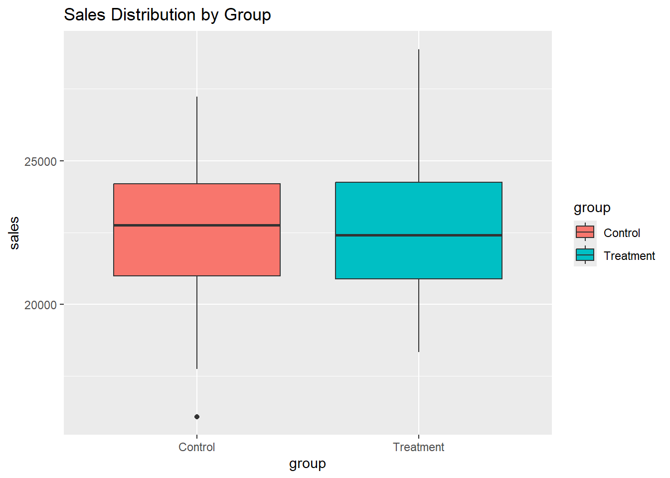
The groups are nearly identical in terms of sale pre-treatment (baseline) and show similar variability.

Code
sales %>%
  filter(period == "Pre")  %>%
  group_by(group, period) %>%
  summarise(mean = mean(sales), 
            sd = sd(sales), 
            median = median(sales))
group period mean sd median
Control Pre 22570.47 2161.540 22750.56
Treatment Pre 22574.74 2169.698 22412.04

The groups are well-balanced and there is no indication of outliers impacting the mean.

Code
sales %>%
  filter(period == "Pre")  %>%
  ggplot(aes(x = group, y = sales, fill = group)) +
  geom_boxplot() +
  labs(title = "Sales Distribution by Group")

Data Wrangling

Since we will be running regression on this data, we create dummy variables for group and period.

Code
sales <- sales %>%
  mutate(
    treatment = case_when( # Create dummy variables for regression
     group == "Treatment" ~ 1, 
     group == "Control" ~ 0),
  post = case_when(
    period == "Post" ~ 1,
    period == "Pre" ~ 0
  )
  )  %>%
  mutate(
    week_fct = as.factor(week), # Create factor variables for regression
    store_id_fct = as.factor(store_id)
  )

DiD Assumptions

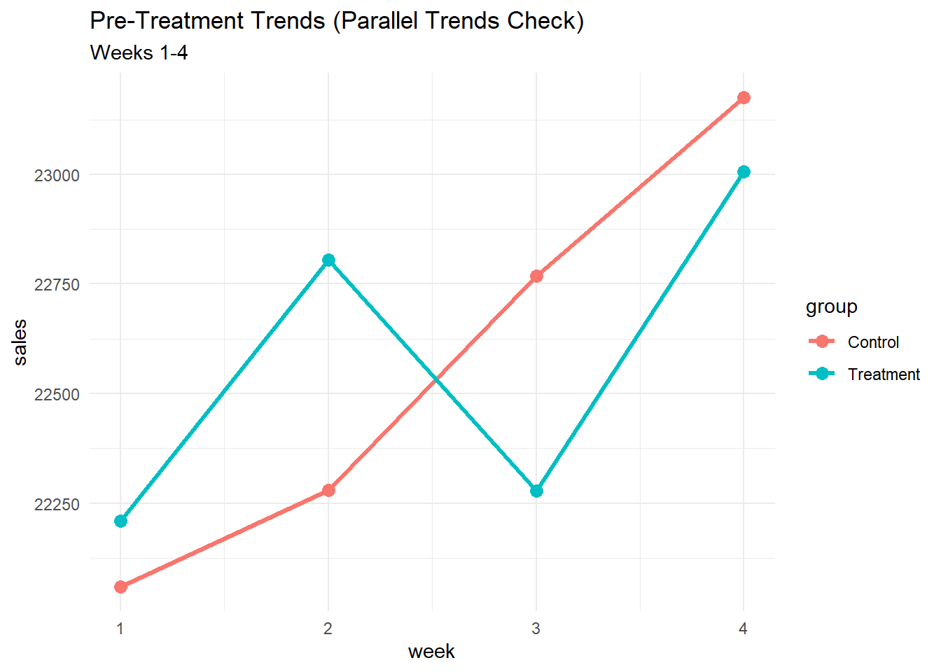
For a differences-in-differences analysis, the existence of parallel is a crucial assumption.

Visual inspection reveals slight non-parallelism in pre-treatment trends, with treatment stores showing more volatility.

Code
pre_data <- sales %>% 
  filter(period == "Pre")

ggplot(pre_data, aes(x = week, y = sales, color = group)) +
  stat_summary(fun = mean, geom = "line", size = 1.2) +
  stat_summary(fun = mean, geom = "point", size = 3) +
  labs(title = "Pre-Treatment Trends (Parallel Trends Check)",
       subtitle = "Weeks 1-4") +
  theme_minimal()

Code
sales %>% 
  filter (period == "Pre")  %>% 
  group_by(group, week)  %>% 
  summarise(sales = sum(sales))
group week sales
Control 1 661760.8
Control 2 668401.4
Control 3 683044.3
Control 4 695249.5
Treatment 1 666273.9
Treatment 2 684138.7
Treatment 3 668358.5
Treatment 4 690198.0

To validate the parallel trends assumption, we regressed pre-treatment sales on treatment status, week, and their interaction. The interaction term was not statistically significant (β = -197.1, p = 0.428), indicating that treatment and control groups followed similar trajectories prior to the intervention. While visual inspection shows some volatility, particularly in the treatment group, these deviations fall within sampling variation and do not invalidate the DiD approach.

Code
pre_model <- lm(sales ~ treatment * week, data = pre_data)
summary(pre_model)  

Call:
lm(formula = sales ~ treatment * week, data = pre_data)

Residuals:
    Min      1Q  Median      3Q     Max 
-5901.4 -1566.5   -70.2  1752.9  6401.4 

Coefficients:
               Estimate Std. Error t value Pr(>|t|)    
(Intercept)     21611.2      480.3  44.994   <2e-16 ***
treatment         496.9      679.3   0.732   0.4652    
week              383.7      175.4   2.188   0.0297 *  
treatment:week   -197.1      248.0  -0.794   0.4277    
---
Signif. codes:  0 '***' 0.001 '**' 0.01 '*' 0.05 '.' 0.1 ' ' 1

Residual standard error: 2148 on 236 degrees of freedom
Multiple R-squared:  0.02447,   Adjusted R-squared:  0.01207 
F-statistic: 1.973 on 3 and 236 DF,  p-value: 0.1187

Checking whether week 4 (last pre-period) shows divergence or not, we find there was no significant difference observed between control and treatment.

Code
t.test(sales ~ group, data = filter(sales, week == 4))

    Welch Two Sample t-test

data:  sales by group
t = 0.31609, df = 57.987, p-value = 0.7531
alternative hypothesis: true difference in means between group Control and group Treatment is not equal to 0
95 percent confidence interval:
 -897.942 1234.708
sample estimates:
  mean in group Control mean in group Treatment 
               23174.98                23006.60 

Finally, we confirm we have complete data for all stores. We’ve observed the same stores throughout the study period, so the composition of our dataset is stable.

Code
sales %>% 
  count(store_id) %>% 
  filter(n != 8)  #filter for stores that have observations different from 8 (duration of experiment)
store_id n

DiD assumptions are met and we can proceed with the analysis.

3 Differences-in-Differences

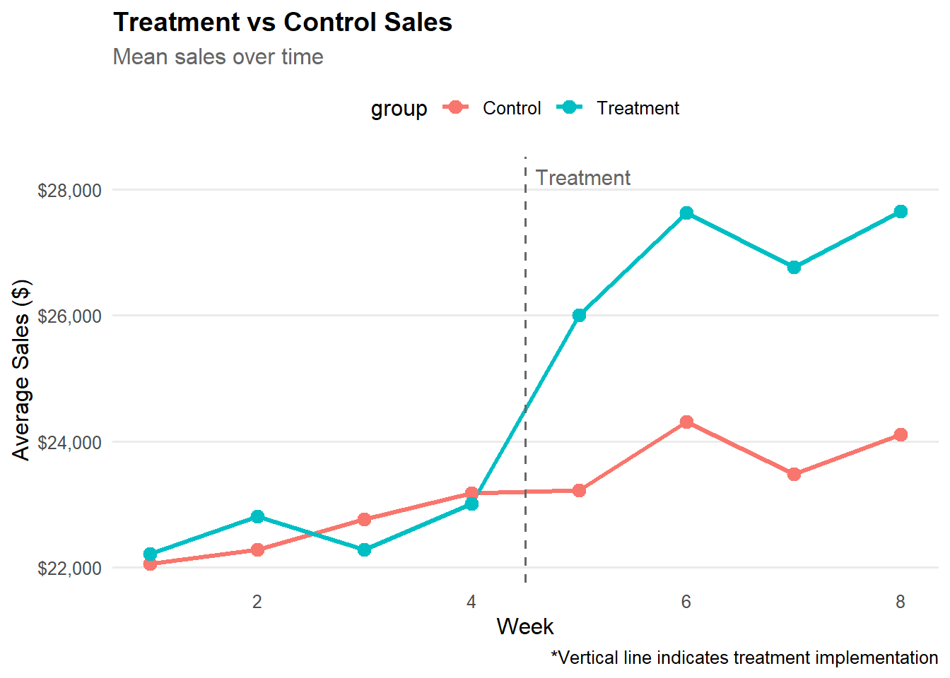
Over time both groups sales are shown to have increased. However, compared to the Control group that serves as our baseline without intervention, the Treatment group has shown a much great increase in sales. With DiD, we will be assessing the impact over time and confirming the difference is not due to random variation.

Code
sales_means <- sales %>%
  group_by(group, week, period) %>%
  summarise(
    mean_sales = mean(sales),
    se = sd(sales) / sqrt(n()),
    .groups = "drop"
  )

ggplot(sales_means, aes(x = week, y = mean_sales, color = group, group = group)) +
  geom_line(size = 1.2) +
  geom_point(size = 3) +
  geom_vline(xintercept = 4.5, linetype = "dashed", color = "gray40") +
  annotate("text", x = 4.5, y = max(sales_means$mean_sales) * 1.02, 
           label = "Treatment", hjust = -0.1, color = "gray40", size = 4) +
  labs(
    title = "Treatment vs Control Sales",
    subtitle = "Mean sales over time",
    x = "Week",
    y = "Average Sales ($)",
    caption = "*Vertical line indicates treatment implementation"
  ) +
  scale_y_continuous(labels = scales::dollar_format()) +
  theme_minimal(base_size = 12) +
  theme(
    plot.title = element_text(face = "bold", size = 14),
    plot.subtitle = element_text(color = "gray40"),
    legend.position = "top",
    panel.grid.minor = element_blank(),
    panel.grid.major.x = element_blank()
  )

4 Model 1 - Without Control Variables

Model 1 estimates DiD by looking at the interaction term treatment * post. Treatment stores sold only $4 more than control at baseline (not significant), confirming once more that groups were balanced before intervention.

Average sales for control group in pre-period is $22,570 and even without treatment, sales increased by $1,210.

However, Treatment stores gained an additional $3,230 beyond the natural trend, which is highly significant (p < 0.001). While both groups experienced sales increases during the post-period, treatment stores gained an additional $3,230 beyond the natural market trend captured by the control group.

This is strong evidence of campaign impact and explains 40% of variation.

Code
model <- lm(sales ~ treatment * post, data = sales)

summary(model)

Call:
lm(formula = sales ~ treatment * post, data = sales)

Residuals:
    Min      1Q  Median      3Q     Max 
-6477.0 -1584.6    46.9  1594.8  6308.1 

Coefficients:
                Estimate Std. Error t value Pr(>|t|)    
(Intercept)    22570.467    202.857 111.263  < 2e-16 ***
treatment          4.276    286.882   0.015    0.988    
post            1210.481    286.882   4.219 2.93e-05 ***
treatment:post  3229.774    405.713   7.961 1.26e-14 ***
---
Signif. codes:  0 '***' 0.001 '**' 0.01 '*' 0.05 '.' 0.1 ' ' 1

Residual standard error: 2222 on 476 degrees of freedom
Multiple R-squared:  0.4028,    Adjusted R-squared:  0.399 
F-statistic:   107 on 3 and 476 DF,  p-value: < 2.2e-16

Model 2 - With Control Variables

We can improve our model by adding fixed effects store_id_fct and week_fct, controlling for baseline differences between stores (e.g location) and time shocks (e.g seasonality). Since DiD is observational data without random assignment, control variable play a crucial role in fitting the model.

Model 2 has increased the adjusted R-squared statistic from 0.4 to 0.81, and therefore is able to explain over 80% of the variation by estimating 97 parameters instead of 4.

Treatment effect also increased from $3,230 to $3,982.

The treatment:post:store_id_fctTXX coefficients show how each treatment store’s effect differs from the $3,982 average Most store-specific interactions are not significant, meaning the treatment effect is fairly homogeneous across stores.

Code
model2 <- lm(sales ~ treatment:post * store_id_fct + week_fct, data = sales)

summary(model2)

Call:
lm(formula = sales ~ treatment:post * store_id_fct + week_fct, 
    data = sales)

Residuals:
    Min      1Q  Median      3Q     Max 
-3330.0  -749.0    11.3   768.8  2955.6 

Coefficients: (30 not defined because of singularities)
                                Estimate Std. Error t value Pr(>|t|)    
(Intercept)                    24193.491    466.040  51.913  < 2e-16 ***
store_id_fctC02                -4655.642    619.098  -7.520 3.93e-13 ***
store_id_fctC03                -1685.300    619.098  -2.722 0.006781 ** 
store_id_fctC04                  727.535    619.098   1.175 0.240664    
store_id_fctC05                -3597.876    619.098  -5.811 1.30e-08 ***
store_id_fctC06                -3715.736    619.098  -6.002 4.53e-09 ***
store_id_fctC07                -1164.183    619.098  -1.880 0.060806 .  
store_id_fctC08                -2275.050    619.098  -3.675 0.000272 ***
store_id_fctC09                -4250.897    619.098  -6.866 2.67e-11 ***
store_id_fctC10                -1651.965    619.098  -2.668 0.007947 ** 
store_id_fctC11                   77.381    619.098   0.125 0.900597    
store_id_fctC12                -2331.401    619.098  -3.766 0.000192 ***
store_id_fctC13                -1478.990    619.098  -2.389 0.017380 *  
store_id_fctC14                -2282.185    619.098  -3.686 0.000260 ***
store_id_fctC15                  932.096    619.098   1.506 0.133002    
store_id_fctC16                -3658.644    619.098  -5.910 7.58e-09 ***
store_id_fctC17                -3180.551    619.098  -5.137 4.45e-07 ***
store_id_fctC18                -1090.210    619.098  -1.761 0.079042 .  
store_id_fctC19                -6256.712    619.098 -10.106  < 2e-16 ***
store_id_fctC20                -1056.365    619.098  -1.706 0.088764 .  
store_id_fctC21                -1351.421    619.098  -2.183 0.029651 *  
store_id_fctC22                -4972.286    619.098  -8.031 1.20e-14 ***
store_id_fctC23                -1836.072    619.098  -2.966 0.003209 ** 
store_id_fctC24                -2594.873    619.098  -4.191 3.45e-05 ***
store_id_fctC25                 -956.014    619.098  -1.544 0.123365    
store_id_fctC26                -1019.104    619.098  -1.646 0.100561    
store_id_fctC27                -2089.431    619.098  -3.375 0.000814 ***
store_id_fctC28                 -930.511    619.098  -1.503 0.133660    
store_id_fctC29                 -532.661    619.098  -0.860 0.390116    
store_id_fctC30                -2974.436    619.098  -4.804 2.23e-06 ***
store_id_fctT01                  237.164    762.438   0.311 0.755924    
store_id_fctT02                -3833.598    762.438  -5.028 7.62e-07 ***
store_id_fctT03                -1689.611    762.438  -2.216 0.027274 *  
store_id_fctT04                -3471.696    762.438  -4.553 7.10e-06 ***
store_id_fctT05                -1074.476    762.438  -1.409 0.159569    
store_id_fctT06                -4553.536    762.438  -5.972 5.34e-09 ***
store_id_fctT07                -1066.701    762.438  -1.399 0.162603    
store_id_fctT08                -1303.461    762.438  -1.710 0.088151 .  
store_id_fctT09                  184.584    762.438   0.242 0.808835    
store_id_fctT10                -4869.798    762.438  -6.387 4.90e-10 ***
store_id_fctT11                -2779.476    762.438  -3.646 0.000304 ***
store_id_fctT12                -1501.711    762.438  -1.970 0.049603 *  
store_id_fctT13                 1437.122    762.438   1.885 0.060200 .  
store_id_fctT14                -2187.236    762.438  -2.869 0.004349 ** 
store_id_fctT15                -2214.043    762.438  -2.904 0.003899 ** 
store_id_fctT16                  947.732    762.438   1.243 0.214618    
store_id_fctT17                -4349.396    762.438  -5.705 2.34e-08 ***
store_id_fctT18                -3300.891    762.438  -4.329 1.91e-05 ***
store_id_fctT19                 -675.691    762.438  -0.886 0.376053    
store_id_fctT20                 -470.008    762.438  -0.616 0.537961    
store_id_fctT21                -4045.206    762.438  -5.306 1.90e-07 ***
store_id_fctT22                -5130.791    762.438  -6.729 6.23e-11 ***
store_id_fctT23                -1555.946    762.438  -2.041 0.041961 *  
store_id_fctT24                -4532.813    762.438  -5.945 6.22e-09 ***
store_id_fctT25                -2840.423    762.438  -3.725 0.000224 ***
store_id_fctT26                  448.164    762.438   0.588 0.557010    
store_id_fctT27                -3789.563    762.438  -4.970 1.01e-06 ***
store_id_fctT28                -2891.156    762.438  -3.792 0.000174 ***
store_id_fctT29                -1593.356    762.438  -2.090 0.037293 *  
store_id_fctT30                  742.594    762.438   0.974 0.330685    
week_fct2                        408.424    226.063   1.807 0.071597 .  
week_fct3                        389.469    226.063   1.723 0.085725 .  
week_fct4                        956.879    226.063   4.233 2.89e-05 ***
week_fct5                        868.373    252.746   3.436 0.000656 ***
week_fct6                       2222.942    252.746   8.795  < 2e-16 ***
week_fct7                       1372.603    252.746   5.431 9.99e-08 ***
week_fct8                       2132.776    252.746   8.438 6.68e-16 ***
treatment:post                  3982.442    890.010   4.475 1.01e-05 ***
treatment:post:store_id_fctC02        NA         NA      NA       NA    
treatment:post:store_id_fctC03        NA         NA      NA       NA    
treatment:post:store_id_fctC04        NA         NA      NA       NA    
treatment:post:store_id_fctC05        NA         NA      NA       NA    
treatment:post:store_id_fctC06        NA         NA      NA       NA    
treatment:post:store_id_fctC07        NA         NA      NA       NA    
treatment:post:store_id_fctC08        NA         NA      NA       NA    
treatment:post:store_id_fctC09        NA         NA      NA       NA    
treatment:post:store_id_fctC10        NA         NA      NA       NA    
treatment:post:store_id_fctC11        NA         NA      NA       NA    
treatment:post:store_id_fctC12        NA         NA      NA       NA    
treatment:post:store_id_fctC13        NA         NA      NA       NA    
treatment:post:store_id_fctC14        NA         NA      NA       NA    
treatment:post:store_id_fctC15        NA         NA      NA       NA    
treatment:post:store_id_fctC16        NA         NA      NA       NA    
treatment:post:store_id_fctC17        NA         NA      NA       NA    
treatment:post:store_id_fctC18        NA         NA      NA       NA    
treatment:post:store_id_fctC19        NA         NA      NA       NA    
treatment:post:store_id_fctC20        NA         NA      NA       NA    
treatment:post:store_id_fctC21        NA         NA      NA       NA    
treatment:post:store_id_fctC22        NA         NA      NA       NA    
treatment:post:store_id_fctC23        NA         NA      NA       NA    
treatment:post:store_id_fctC24        NA         NA      NA       NA    
treatment:post:store_id_fctC25        NA         NA      NA       NA    
treatment:post:store_id_fctC26        NA         NA      NA       NA    
treatment:post:store_id_fctC27        NA         NA      NA       NA    
treatment:post:store_id_fctC28        NA         NA      NA       NA    
treatment:post:store_id_fctC29        NA         NA      NA       NA    
treatment:post:store_id_fctC30        NA         NA      NA       NA    
treatment:post:store_id_fctT01   528.375   1238.196   0.427 0.669816    
treatment:post:store_id_fctT02 -1073.918   1238.196  -0.867 0.386308    
treatment:post:store_id_fctT03   -91.210   1238.196  -0.074 0.941317    
treatment:post:store_id_fctT04  -683.833   1238.196  -0.552 0.581078    
treatment:post:store_id_fctT05 -1131.640   1238.196  -0.914 0.361322    
treatment:post:store_id_fctT06   672.355   1238.196   0.543 0.587438    
treatment:post:store_id_fctT07 -1084.140   1238.196  -0.876 0.381807    
treatment:post:store_id_fctT08 -1743.992   1238.196  -1.408 0.159796    
treatment:post:store_id_fctT09 -2588.243   1238.196  -2.090 0.037247 *  
treatment:post:store_id_fctT10 -1741.467   1238.196  -1.406 0.160400    
treatment:post:store_id_fctT11  -666.537   1238.196  -0.538 0.590673    
treatment:post:store_id_fctT12   529.838   1238.196   0.428 0.668957    
treatment:post:store_id_fctT13   852.123   1238.196   0.688 0.491746    
treatment:post:store_id_fctT14  -409.510   1238.196  -0.331 0.741028    
treatment:post:store_id_fctT15 -1476.402   1238.196  -1.192 0.233850    
treatment:post:store_id_fctT16  -602.962   1238.196  -0.487 0.626559    
treatment:post:store_id_fctT17  -907.370   1238.196  -0.733 0.464119    
treatment:post:store_id_fctT18 -2080.710   1238.196  -1.680 0.093688 .  
treatment:post:store_id_fctT19 -1055.512   1238.196  -0.852 0.394492    
treatment:post:store_id_fctT20  -576.597   1238.196  -0.466 0.641713    
treatment:post:store_id_fctT21 -2081.562   1238.196  -1.681 0.093554 .  
treatment:post:store_id_fctT22   391.973   1238.196   0.317 0.751744    
treatment:post:store_id_fctT23 -2006.085   1238.196  -1.620 0.106019    
treatment:post:store_id_fctT24  -967.810   1238.196  -0.782 0.434916    
treatment:post:store_id_fctT25 -1268.712   1238.196  -1.025 0.306177    
treatment:post:store_id_fctT26   244.275   1238.196   0.197 0.843711    
treatment:post:store_id_fctT27     5.428   1238.196   0.004 0.996505    
treatment:post:store_id_fctT28  -591.757   1238.196  -0.478 0.632981    
treatment:post:store_id_fctT29  -974.415   1238.196  -0.787 0.431790    
treatment:post:store_id_fctT30        NA         NA      NA       NA    
---
Signif. codes:  0 '***' 0.001 '**' 0.01 '*' 0.05 '.' 0.1 ' ' 1

Residual standard error: 1238 on 383 degrees of freedom
Multiple R-squared:  0.8508,    Adjusted R-squared:  0.8134 
F-statistic: 22.75 on 96 and 383 DF,  p-value: < 2.2e-16

Discussion

The consistency of high treatment effect ($3,230 vs $3,982) and low p-values (p < 0.001) demonstrates the campaign’s positive impact is robust across model specifications. That said, the inclusion of confounders is shown to greatly improve model fit (0.4 vs 0.81).

Model 1 is shown to have omitted variable bias:

  • Doesn’t account for high-performing vs low-performing stores

  • Doesn’t control for week-to-week variation (e.g., week 6 had big sales boost)

  • Treatment effect is “contaminated” by these confounders

On the other hand, Model 2 isolates the true effect by comparing:

  • Each store to itself (within-store comparison)

  • Same week across groups (within-week comparison)

Model 2 should be preferred for estimating the outcome.

5 Campaign Impact

Based on Model 2, the incremental revenue generated by the treatment is as follows:

  • Per store per week: $3,982

  • Per store (4 weeks): $15,930

  • Total (30 stores): $477,389

Code
# Extract treatment effect from Model 2
treatment_effect <- 3982.442  # Average treatment effect (treatment:post coefficient)

# Study parameters
n_treatment_stores <- 30
n_post_weeks <- 4

# Calculate incremental revenue
revenue_per_store_per_week <- treatment_effect
revenue_per_store_total <- revenue_per_store_per_week * n_post_weeks
total_incremental_revenue <- revenue_per_store_total * n_treatment_stores

revenue_per_store_per_week
[1] 3982.442
Code
revenue_per_store_total
[1] 15929.77
Code
total_incremental_revenue
[1] 477893

6 Conclusion

This difference-in-differences analysis demonstrates that the sales campaign generated a significant and substantial impact. Treatment stores experienced an average increase of $3,982 per week compared to control stores, representing approximately $477,000 in incremental revenue across 30 stores over the four-week post-campaign period. This effect remained highly significant (p < 0.001) even after controlling for baseline store differences and weekly market fluctuations, providing strong evidence of the campaign’s causal impact.

Critically, the treatment effect proved consistent across nearly all stores, with only one location showing a significantly different response. This homogeneity indicates the campaign is scalable and replicable. Marketing teams can confidently deploy this strategy to additional locations with predictable results.

The fixed effects model (Model 2) substantially outperformed the simple difference-in-differences specification, explaining 81% of sales variation compared to just 40% in the basic model. By isolating the true campaign effect from confounding factors like store size, location advantages, and seasonal timing, Model 2 provides the most credible estimate for business decision-making. The robustness of results across specifications—ranging from $3,230 to $3,982 depending on controls—further validates the campaign’s effectiveness and supports broader implementation.