---
title: "Churn Prediction with Tidymodels - Part 2: Random Forest"
author: Ceren Unal
#date:
categories: [classification]
image: image-man-watching-tv.png
description: The second part of the Churn Prediction project builds a Random Forest model using that outperforms the baseline model.
toc: true
toc-title: Content
toc-location: right
number-sections: true
number-depth: 2
smooth-scroll: true
df-print: kable
code-fold: true
code-tools: true
code-overflow: wrap
code-block-bg: true
code-block-border-left: "#31BAE9"
highlight-style: pygments
code-link: true
execute:
warning: false
message: false
#comments:
# hypothesis: true
---
In Part 1, I developed a benchmark churn prediction model for Skystream using the K-Nearest Neighbors (KNN) algorithm. The KNN model correctly identified 47% of all churn cases, achieving a precision of 57%.
In Part 2 the goal is to build a Random Forest model that outperforms KNN on imbalanced, high-dimensional data, with a focus on improving both recall and precision.
## Load Packages & Data
We will be using the Tidyverse package to process our data set. As in Part 1, I will clean up the incorrect namings in the Genre variable and create a Churn variable based on CancelDate.
```{r}
library(tidyverse)
library(DataExplorer)

skystream <- read_csv(file = "skystream.csv")

skystream <- skystream|>
  mutate(
    churn = if_else(is.na(CancelDate), 0L, 1L) #return 1 if there is a CancelDate
  ) %>%
  relocate(churn, .after = 1) |>  #position it after column 1
  mutate(Genre = recode(Genre, "Dramas" = "Drama")) #replace Dramas with Drama

head(skystream)
```
## Data Preparation for Random Forest
We'll prepare our data for Random Forest by ensuring that all continuous variables are numeric and we drop the variables that we won't be using in our model. RevenueYTD is dropped as it would be reduntant when we have both SubscriptionTier and NumberMonthsActive in the model, which directly determine this 3rd variable.
We'll convert the Churn variable, which indicates whether a customer has churned, into a factor so it can be treated as a categorical classification outcome.
The categorical variables will be recoded as dummy variables.
```{r}
library(fastDummies)
library(snakecase)

# Define columns by role/type
num_cols  <- c("NumberMonthsActive", "AvgSessionLength", "Age",
               "MonthsSinceLastActivity", "AvgWatchHoursPerMonth")

cat_cols  <- c("SubscriptionTier", "Genre", "State", "Gender", "DevicePreference")

skystream_rf <- skystream |>
  #Make “Churned” the first level so tidymodels treats Churned as the positive class
  mutate(churn = factor(churn, levels = c(1, 0), labels = c("Churned", "Active"))) |>

  # Ensure numericals are numeric
   mutate(across(all_of(num_cols), as.numeric)) |>

  # Remove columns not suitable as KNN features
  select(-CustomerID, -JoinDate, -CancelDate, -RevenueYTD) |>

  # One-hot encode categoricals (drop first level to avoid redundancy)
  fastDummies::dummy_cols(
    select_columns = cat_cols,
    remove_first_dummy = TRUE,
    remove_selected_columns = TRUE
  ) %>%

  #Ensure column names are all in tidy format
   rename_with(~ to_any_case(., case = "upper_camel"))
```
## Creating the Model
We set the seed to 867, the same as KNN, to ensure the observations are random and consistent across both models. We use `initial_split()` to divide the dataset, with 80% allocated for training and 20% for testing. Then, we use the `strata = churned` argument to ensure the class distribution of the churned variable is kept in both the training and testing sets. Finally, we extract the datasets for training and testing using split.
```{r}
library(tidymodels)
library(themis)

set.seed(867)
Split80  <- initial_split(skystream_rf, prop = 0.80, strata = Churn)

DataTrain <- training(Split80)
DataTest  <- testing(Split80)

head(DataTrain)
```
As with KNN, we specify the recipe with Churn \~ ., which means all other columns, such as Age and NumberMonthsActive, will be used to predict whether a customer churned.
```{r}
RecipeRF <- recipe(Churn~., data=DataTrain)
```
The model design specifies `min_n` and `mtry` as tunable hyperparameters and sets the number of trees to 2,000 for increased stability. The model is configured to run using the `"ranger"` engine and the `importance = "impurity"` argument enables the calculation of variable importance scores, helping identify which features contribute most to churn prediction. Setting `probability = TRUE` ensures that class probabilities are returned (not just hard predictions), which is required for ROC AUC and threshold optimization. Finally, `num.threads = detectCores()` allows the model to use all available processor cores to speed up computation, and `set_mode("classification")` confirms the task is binary classification (churn vs. active).
```{r}
library(parallel)
ModelDesignRandFor <- rand_forest(
  min_n=tune(),
  mtry=tune(),
  trees=2000) |>
  set_engine("ranger",
             importance = "impurity", #generate variable importance plots
             probability = TRUE, #generate class probabilities
             num.threads=detectCores()) |> #set as number of cores of the executing computer
  set_mode("classification")

set.seed(123)
WfModelRF=workflow() |>
           add_recipe(RecipeRF) |>
           add_model(ModelDesignRandFor)
```
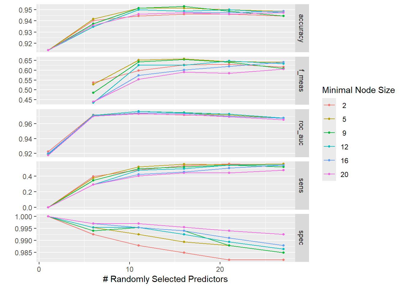
We'll tune `min_n` and `mtry` using a regular tuning grid created with `grid_regular()`, which generates 36 combinations of `mtry` (number of predictors sampled at each tree split) and `min_n` (minimum node size), evenly spaced across defined ranges. The `finalize(mtry(), ...)` function ensures that `mtry` adapts to the actual number of predictors in the training data.
Cross-validation is set up using `vfold_cv()` with 5 folds, stratified by the target variable `Churn` to preserve class balance in each fold. The `tune_grid()` function evaluates each hyperparameter combination using cross-validation and saves the class probabilities for later threshold tuning. A comprehensive metric set is used—including ROC AUC, accuracy, sensitivity, specificity, and F1 score—to assess both overall and class-specific performance.
```{r}
#| warning: false
rf_grid <- grid_regular(
  finalize(mtry(), DataTrain |> select(-Churn)),  # mtry depends on predictors
  min_n(range = c(2L, 20L)),
  levels = c(6, 6)   #36 configs
)

set.seed(123)

FoldsForTuningRF=vfold_cv(DataTrain, v=5, strata=Churn)

rf_tune <- tune_grid(
  WfModelRF,
  resamples = FoldsForTuningRF,
  grid = rf_grid,
  metrics = metric_set(roc_auc, accuracy, sens, spec, f_meas),
  control = control_grid(save_pred = TRUE)
)

autoplot(rf_tune)
```
The best hyperparameters are 16 for `mtry` and 9 for `min_n` , based on the ROC AUC metric finds the optimal balance between true positive rate and false positive rate.
```{r}
best_rf <- select_best(rf_tune, metric = "roc_auc")

best_rf
```
After running the best hyper parameters, we go ahead and take a look at our confusion matrix to assess model performance.
```{r}
WFModelBest=WfModelRF |>
  finalize_workflow(best_rf) |>
  fit(DataTrain)

PredictionBestModel=augment(WFModelBest, DataTest)

cm_rf <- conf_mat(PredictionBestModel, truth=Churn,
         estimate=.pred_class)

library(yardstick)

cm_rf
cm_rf %>% summary()
```
Random Forest is already outperforming KNN, with 86% recall and 86% precision, compared to 47% recall and 57% precision.
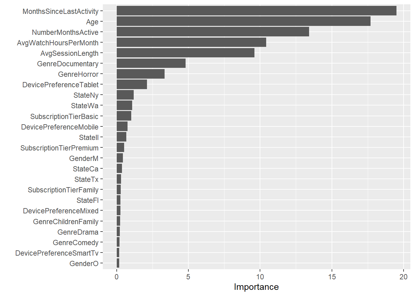
Variable importance in our model reveals that `MonthsSinceLastActivity` was the biggest predictor of `Churn`.
```{r}
library(vip)
rf_fit <- WFModelBest |>
          extract_fit_parsnip()
vip(rf_fit$fit, num_features = 25)
```
## Refining the Model
### **Thresholds**
To further improve the recall and precision of our model, we'll try adjusting our threshold.
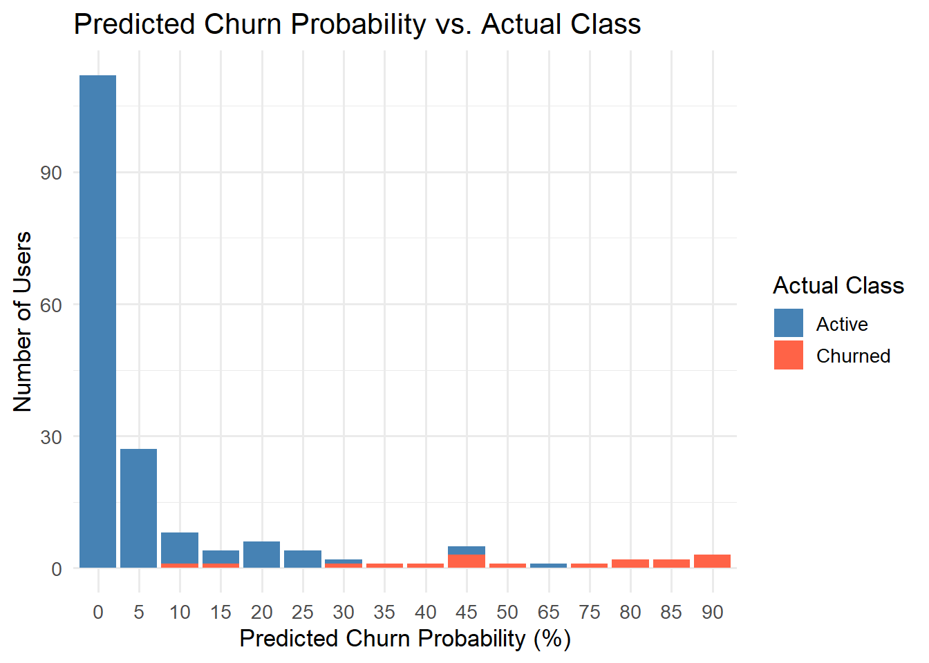
After scanning a range of thresholds we find that the range of values from 0.47 to 0.5 maximizes F1 score, so the default threshold that we initially tuned our model to already maximized F1 score.
This is evident in that when we drop the threshold to 0.48, the recall and precision (along with all other metrics) remain the same.
```{r}
# Try thresholds from 0.05 to 0.95
ths <- seq(0.05, 0.95, by = 0.01)

scan_f1 <- map_dfr(ths, function(t) {
  cls <- factor(
    ifelse(PredictionBestModel$.pred_Churned >= t, "Churned", "Active"),
    levels = c("Churned","Active")
  )
  tibble(
    threshold = t,
    f1 = f_meas_vec(PredictionBestModel$Churn, cls, beta = 1),
    precision = precision_vec(PredictionBestModel$Churn, cls),
    recall = sens_vec(PredictionBestModel$Churn, cls)
  )
})

# Show the best threshold by F1
best_thresh_f1 <- scan_f1 |>
  slice_max(f1, n = 1)  |>
  pull(threshold)

best_thresh_f1
PredictionBestModel_f1 <- PredictionBestModel  |>
  mutate(
    .pred_class_opt = factor(
      ifelse(.pred_Churned >= 0.48, "Churned", "Active"),
      levels = c("Churned","Active")
    )
  )

cm_rf_f1 <- conf_mat(PredictionBestModel_f1, truth = Churn, estimate = .pred_class_opt)

cm_rf_f1  |>
  summary()
```
```{r}
plot_data <- PredictionBestModel_f1|>
  select(.pred_Churned, Churn) |>
  mutate(Churn = factor(Churn, levels = c("Active", "Churned"))) |>
  mutate(ProbBin = round(100 * .pred_Churned / 5) * 5) |>
  count(ProbBin, Churn) |>
  pivot_wider(names_from = Churn, values_from = n, values_fill = 0) |>
  pivot_longer(cols = c("Active", "Churned"), names_to = "Class", values_to = "Count")


ggplot(plot_data, aes(x = factor(ProbBin), y = Count, fill = Class)) +
  geom_col(position = "stack", width = 0.9) +
  scale_fill_manual(values = c("Active" = "steelblue", "Churned" = "tomato")) +
  labs(
    title = "Predicted Churn Probability vs. Actual Class",
    x = "Predicted Churn Probability (%)",
    y = "Number of Users",
    fill = "Actual Class"
  ) +
  theme_minimal(base_size = 13)
```
## Conclusion
The Random Forest model demonstrated strong predictive performance in identifying customer churn. After tuning the model using ROC AUC and optimizing the classification threshold for F1, it achieved balanced and reliable results — with precision and recall both around 0.86 and an overall F1 score of 0.83. This means the model correctly identifies the majority of churners while maintaining a low rate of false positives.
Compared to earlier approaches, such as KNN, Random Forest provided superior accuracy, stability, and interpretability through feature importance. Overall, the model offers a robust and actionable framework for predicting churn risk, enabling the business to focus retention efforts on the customers most likely to leave.